System Dynamics Applications / F / F.9

F.9 MODULE—DELAYED INFLOW

F.9.1 General Description

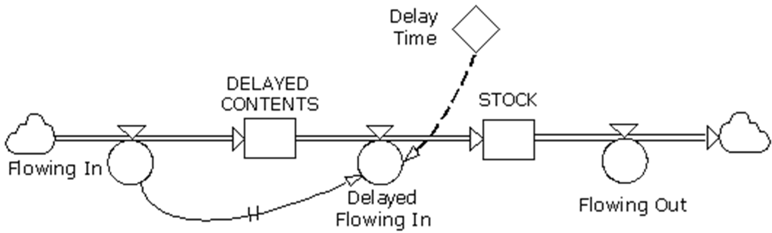
Items (or quantities of material) arrive from outside the defined problem space. These are added to the DELAYED CONTENTS, but inflow to STOCK cannot take place immediately. Inflow to the stock of primary interest, STOCK is delayed.

Both Sterman (2000: 464-5) and Coyle (1996: 98-108) caution us that when building system dynamics models we need to be very clear of exactly the type of delay mechanism that operates. Unless otherwise specified in first order delays, the stock of material in transit are perfectly mixed at all times, meaning that outputs from DELAY CONTENTS are in random order with respect to their input. In higher order delays material is output in the same order as they are input; the order depends on the number of process stages involved. These diagrams do not specify the type of delay mechanism.

Delay Time is used to set the length of delay (and a variety of types of delay may be involved, though a pipeline delay is represented here). The rate-controlling auxiliaries at either side of DELAYED CONTENTS are linked. This might be specified as a pipeline delay as described in the module First-order (Pipeline) Delay. Items, or material, flow out of STOCK and across the module boundary according to separate governing business rules.

F.9.2 Influence Diagram Representation

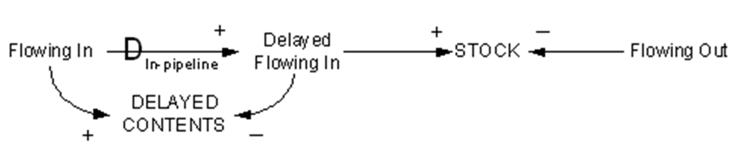
The influence diagram representation for this module is shown in Figure F9-2.

F.9.3 Reference Sources

This module is described after Coyle (1996: 38). Delays are described in Sterman (2000: Ch 11) and in the Powersim™ Studio Reference Guide.

F.9.4 Application

Delays occur where output does not instantaneously follow an input to a stock. The form of the delay can vary from exact reproduction (which is the case for a higher-order pipeline delay) to output growing to the value of the input, where growth takes time be fully realised (which is the case for an information delay).

The rate control valves at either side of the accumulator titled DELAY CONTENTS are linked. The solid arrow with the two bars across it, confirms that Flowing In and Delayed Flowing In rate-controlling variables are linked by a specified delay.

This module forms the basis for representing delays in a wide range of model types. These include processing delays, delivery lags in supply chain models, population ageing and career succession modelling. An example of a pipeline delay is provided in Figure 5-2.

This module might be used to analyse the impact of delays in the processing of invoices, payment into a bank account and subsequent withdrawals from that account. Once each week, a contractor submits invoices to his client for work the contractor completed during the preceding week. The client normally pays invoices 28 days after receiving them, that is, the Delay Time is 28 days. The contractor withdraws sufficient funds from his bank account each week to pay the salaries of his workforce. Clearly, he cannot make payments if his bank account STOCK has insufficient money in it. In the situation depicted, because the delay time is quite long the contractor is concerned about running into cash flow problems. The contractor would want to know the health of his bank account, wishing to manage it such that it would always contain sufficient funds to accommodate fluctuations exacerbated by invoice-processing delays. When the current contract is due for renewal, the contractor may consider negotiating an arrangement whereby invoices are processed within 14 days instead of 28 days. The contractor might also consider paying a premium for the surety he might enjoy in managing his cash flow.

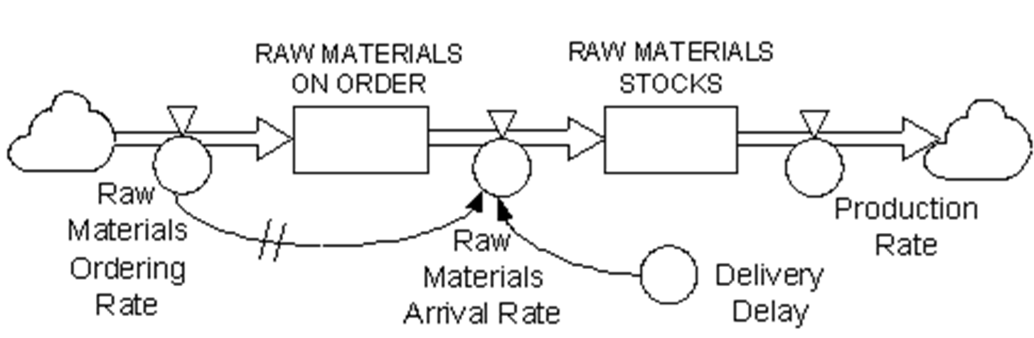
Another example of Delayed Inflow might be that which occurs as materials are ordered to support a firm’s production process. Raw materials are ordered at a particular rate, Raw Material Ordering Rate. Raw materials arrive after a delivery delay time D_DEL. The raw materials are added to existing stocks. All the time, Production Rate is depleting Raw Material Stocks. This is depicted as an influence diagram at Figure F9-3. The equivalent stock-and-flow diagram would be as shown at Figure 9-4.

F.9.5 Functional Description

The functions of the variables contained in the module are described in Table F9-1.

Table F9-1. Functional Description—Delayed Inflow

References

- Sterman, J.D., 2000, Business Dynamics: Systems Thinking and Modelling for a Complex World, Irwin McGraw-Hill.
- Coyle, R.G., 1996, System Dynamics Modelling: A Practical Approach, Chapman and Hall, London.