
F.5 MODULE—FIRST ORDER LINEAR POSITIVE FEEDBACK
F.5.1 General Description
A first-order system contains only one stock (level or accumulator). Systems are described as linear systems when the algebraic expressions controlling rate(s) of flow into the system, that is, creating a change (at any point in time) in the state variable ‘S’ STATE OF SYSTEM are simply the product of a constant and the current value of S. Rate of change of state is:
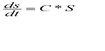
where:
C = a constant, and
S = state of the system
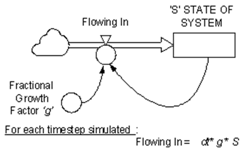
A first-order positive feedback loop has the effect (each time we calculate it) of adding to S an amount (where the constant is a Fractional Growth Factor ‘g’) which is larger than the previous time we calculated it. Consider a series of calculations at times t0, t1, t2 … tn, with the initial value of S being S0 and a Fractional Growth Factor g operating on the inflow. The state of the system will change as shown in Table 5-1.
Table F5-1. Change of State with Time—First-order Linear Positive Feedback
tn | Current State ‘S’ | Net Change of State |
|---|---|---|
0 | S0 | 0 |
1 | S 1 = S0 + g* S0 | g* S0 |
2 | S2 = S0 + g*( S0 + g* S0 ) S2 = S0 + g*( S 1 ) | g*( S 1 ) |
3 | S3 = S0 + g* (S0 + g*( S0 + g* S0 ) ) S3 = S0 + g*( S 2 ) | g*( S 2 ) |
… | ||
n | Sn = S0 + g*( S n-1 ) | g*( S n-1 ) |
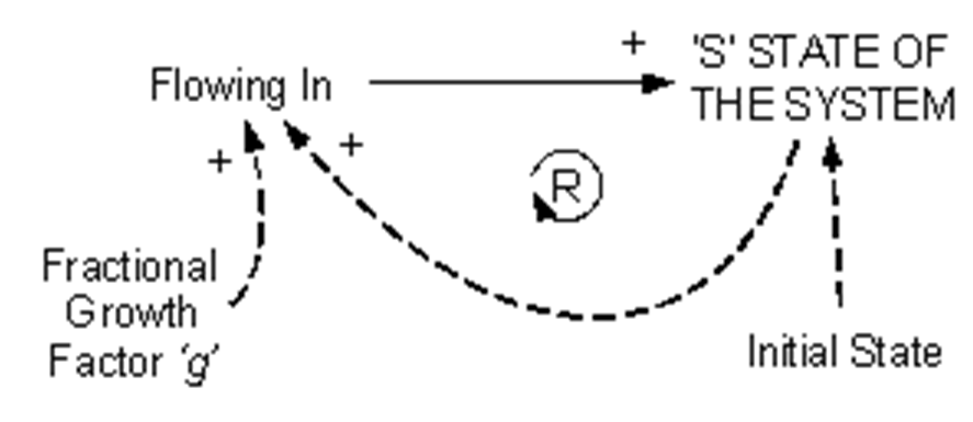
The positive (reinforcing) feedback loop has the effect of accumulating the net inflow rate, that is, the net change of state calculated at each time-step.
F.5.2 Module Influence Diagram
The influence diagram for this module is shown in Figure F5-2.
F.5.3 Reference Sources
This module is described here after Goodman (1989: 18-23) and Sterman (2000: 266). Further explanation of this module can be found at Sterman (2000: 266).
F.5.4 Application
An example might be a bank account with CURRENT BALANCE depending, of course, upon the starting balance, Initial Balance, or initial deposit and an Interest Growth Factor ‘i’. In this simple example, there are no periodic deposits except for the initial deposit when the account was opened.
F.5.5 Example Influence Diagram
The influence diagram is shown in Figure F5-3. The stock-and-flow diagram is shown in Figure F5-4.
F.5.6 Functional Description
The functions of the various parts of the module are described in Table F5-2.
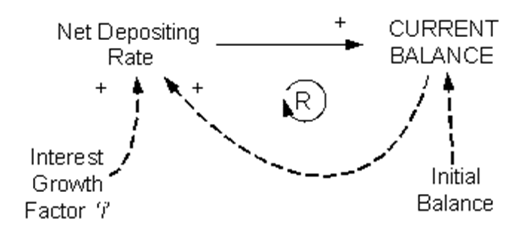
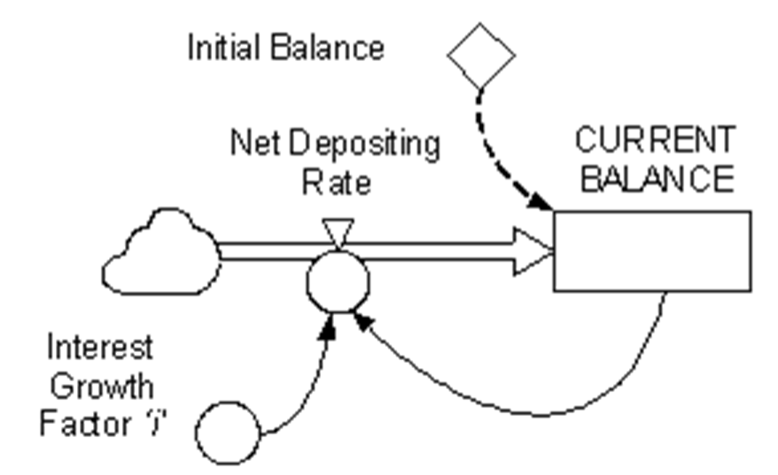
Table F5-2. Functional Description—First-order Linear Positive Feedback—CURRENT BALANCE Example
Variable | Function | Comment |
|---|---|---|
Interest Growth Factor ‘i’ | 10% | This is the interest rate expressed as a percentage. This will be the factor used in the calculating of compounding interest. Units will be expressed as ‘% per interest period’. |
Net Depositing Rate | CURRENT BALANCE * i | In this model, interest is added in increments via the flow valve controlled by the auxiliary variable Net Depositing Rate. Net Depositing Rate will add incremental amounts (each dt) equal to CURRENT BALANCE * i. When dt is infinitesimally small, additions to CURRENT BALANCE occur continuously. Under these conditions, net inflow rate becomes
In this type of example, Powersim™ Studio automatically divides by dt to produce i/dt, to maintain the integrity of the units of the simulation. However, the modeller must be aware of the implications of selecting dt. Unfortunately, Powersim™ Studio does not force the modeller to thinks about dt and timestep as separate entities. Interest rates are generally quoted on a yearly (per annum) basis. However, many financial institutions calculate interest daily. In that instance timestep = 1 year whilst dt = 1 day. |
Initial Balance | $5,000 | An amount of $5,000 is added to an otherwise empty account at the beginning of the simulation. This occurs once only (at the start of the simulation) and is the opening balance added when TIME = 0, before calculations are made at the first instance of dt. The first incremental addition to CURRENT BALANCE is calculated as $5,000 * 0.1 = $500, if interest was to be calculated only once each year and interest added to the bank balance at that time, it dt = TIMESTEP = 1 year. Generally speaking, this initial addition is calculated as: Initial Balance * (Interest Growth Factor/dt) and at any time, after n simulation steps, CURRENT BALANCE = Initial Balance * (1+ Interest Growth Factor/dt)n * dt |
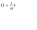 , which approaches
  . If i= 0.1, per interest period and interest is calculated daily (timestep and dt are both set to 1 day);
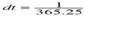 ;
;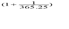 = 1.00027379.
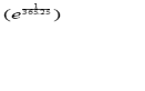 = 1.00027382
References
- Goodman, M.R., 1989, Study Notes in System Dynamics, Productivity Press, Portland, Oregon.
- Sterman, J.D., 2000, Business Dynamics: Systems Thinking and Modelling for a Complex World, Irwin McGraw-Hill.