3.1.4 Determining Contributions To Bathtub Made By Flowing In
The contribution to BATHTUB resulting from Flowing In is determined by calculating the area under the Flowing In curve, as depicted in Figure 3-9, for each increment of time of the simulation. The results are shown in Figure 3-10.
How these were calculated using simple trigonometry is shown in Figures 3-11 and 3-12.
As shown at Figure 3-10, the calculation of the areas under the curve A1, A2 and A6 is trivial for the first, second and sixth elapsed minutes respectively. For the seventh minute and beyond, to the end of the simulation, each of these areas under the curve is zero.
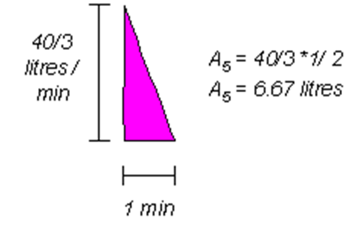
For A5 the area under the curve is a triangle, as shown in Figure 3-11.
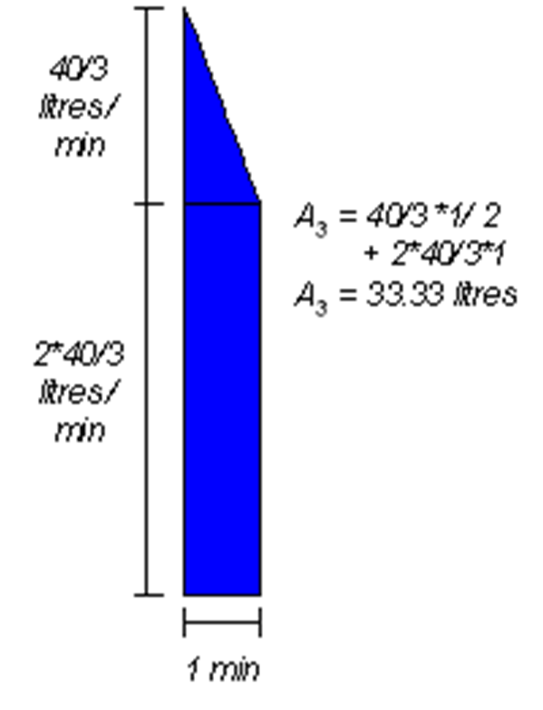
For A3 and A4, the area under the curve comprises a triangle of the same size as shown in Figure 3-11, and a rectangle. For A3 the rectangle is larger than A4. The method used for calculating A3 is shown in Figure 3-12. The method for calculating A4 is the same.
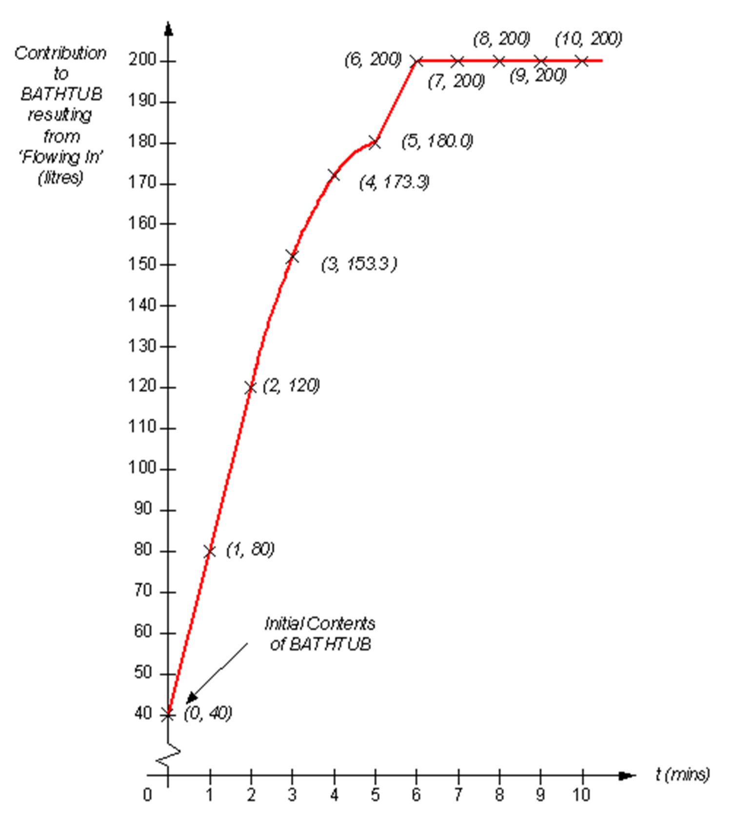
Based on the results of calculating each of the incremental areas, as shown in Figure 3-10, the contribution to BATHTUB resulting from Flowing In is then calculated. The cumulative results are depicted diagrammatically in Figure 3-13.
When calculating the influence of a rate variable on a state variable (for example influence of Flowing In on BATHTUB), the shape of the curve representing change in the state variable is related directly to that of the rate variable. The new graph of the state variable represents the mathematical integration of the rate variable with time.
The results of mathematical integration lead us to observe that:
- Constant rates of inflow produce linear growth. An example of this can be found by considering the first and second minutes in Figures 3-10 and 3-13 respectively. Similarly, we would expect that constant rates of outflow (Flowing Out—the influencing variable) produce linear decline in the state variable (BATHTUB—the influenced variable).
- Linear decreasing rates of inflow alone produce quadratic changes in state (represented by curves which increase in value but have progressively decreasing slope). An example of a linear decreasing rate of inflow can be seen in the third, fourth and fifth minutes of Figure 3-10. This produces a quadratic change (increasing, but with progressively less slope) in the third, fourth and fifth minutes of Figure 3-13. Similarly, we would expect linear increasing rates of inflow alone produce quadratic increasing changes in state (represented by curves which have progressively more slope).
- Zero rates of either inflow or outflow produce zero change in state variables.
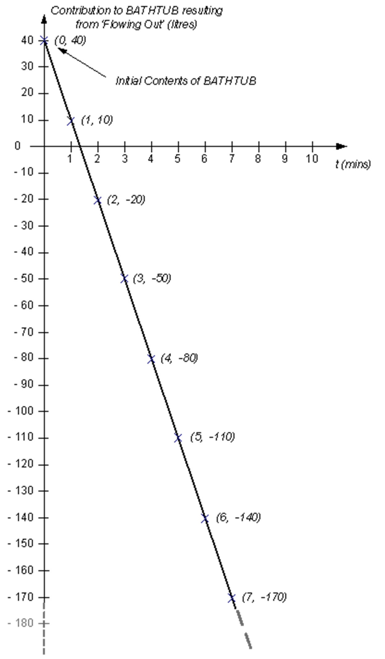
The contribution to BATHTUB resulting from Flowing Out (negative in its sense) is depicted diagrammatically in Figure 3-14.
Whilst the contents of the bathtub cannot become less than zero (at least in an absolute physical sense) it is easy enough to overlook the requirement to constrain flows in a quantitative model so that flows out do not continue when there is no water available. When creating the algebraic relationships in a computational model, we must consciously guard against the possibility that water will be removed (by our model) even when there is none to be removed.
The graphs Figure 3-13 and Figure 3-14 are combined through arithmetic addition to determine the net effect on the contents of BATHTUB.
The sequence of calculation to determine the value of BATHTUB may not seem important at this stage. However, it will be demonstrated in other chapters that the sequence of calculation each increment in time, dt, can be very important. As a general rule, inflows (which increase a state variable) are calculated before outflows (that decrease a state variable) are calculated.
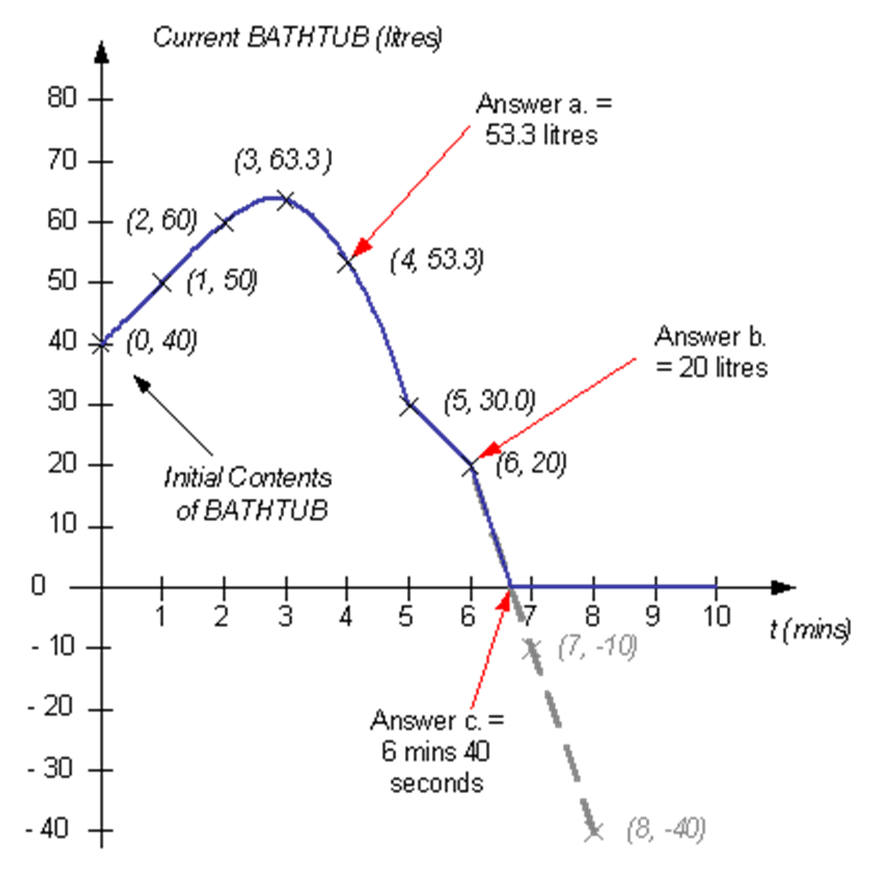
The results are in Table 3-1 and depicted at diagrammatically in Figure 3-15. Note that the quantity of water in the bathtub is not permitted to become negative. The highlighted values of BATHTUB in Table 3-1 are replaced by zeros. The effect of doing this is shown in Figure 3-15 in the form of a dashed line that continues below the time axis.
The results of each of the questions posed earlier now can be read directly from the graph in Figure 3-15:
- 53.3 litres.
- 20.0 litres.
- 6 minutes 40 seconds (6.66 minutes—determined by interpolation of values of Current BATHTUB at 6 minutes and 7 minutes, respectively).
Table 3-1. Calculation of Values for BATHTUB at Each Minute of Elapsed Time
Time (mins) | 0 | 1 | 2 | 3 | 4 | 5 | 6 | 7 | 8 | 9 | 10 |
|---|---|---|---|---|---|---|---|---|---|---|---|
Initial Contents Plus Flowing In | 40 | 80 | 120 | 153.3 | 173.3 | 180 | 200 | 200 | 200 | 200 | 200 |
Initial Contents Less Flowing Out | 40 | 10 | -20 | -50 | -80 | -110 | -140 | -170 | -200 | -230 | -260 |
Sum | 80 | 90 | 100 | 103.33 | 93.33 | 70 | 60 | 30 | 0 | -30 | -60 |
Initial BATHTUB | 40 | 40 | 40 | 40 | 40 | 40 | 40 | 40 | 40 | 40 | 40 |
BATHTUB (litres) | 40 | 50 | 60 | 63.33 | 53.33 | 30 | 20 | –10 | –40 | –70 | –100 |