System Dynamics Applications / 1 / 1.1 / 1.1.3

1.1.3 A Simple Bank Account Example

Consider another example which starts out as being deceptively simple but quickly becomes complex. Imagine that you open a bank account with the intention of saving sufficient for a deposit for an apartment, a house or to buy a new car. You open the account with a starting deposit of $1,000 and plan to make regular deposits of $1,000 each month for a period of three years. The bank pays compounding interest at a rate of 10% per annum. There are no account-keeping charges.

The analysis of such a problem is based on a fundamental principle; the time-value-of-money. This principle says that, for example, if a 10% per annum interest rate prevails we feel totally indifferent to having $1.00 today or $1.10 in a year’s time. Interest rate is also called the discount rate because the $1.10 we might have at the end of a year is actually $1.00 in today’s dollar terms. The term discount is used to suggest that the latter, the amount we might have in our hands today, is less; it has been discounted or reduced in size. In general terms, this principle tells us that a future sum is related to the present sum by the relationship:

F = P (1 + i)ⁿ

where F is the future sum, P is the present sum or principal, i is the interest rate or discount rate per period, and n is the number of periods.

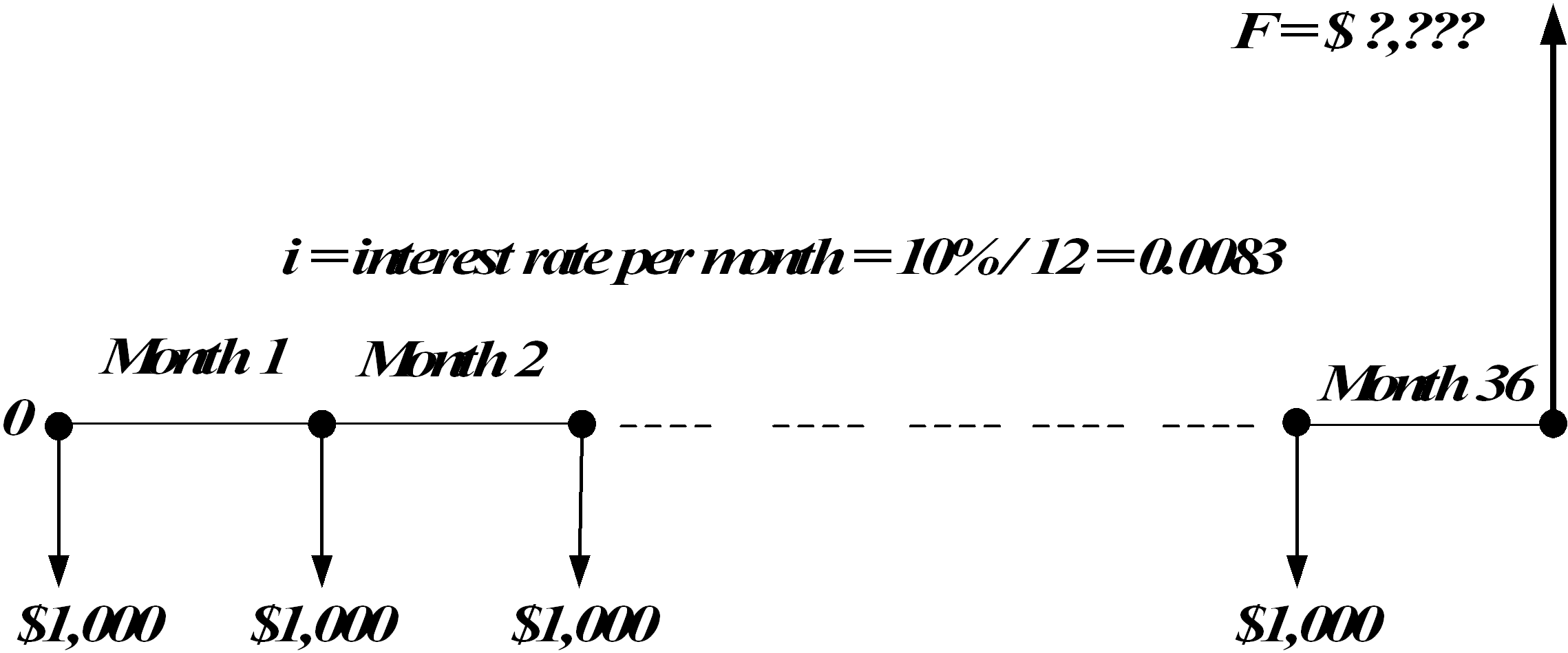
In this example, we wish to make regular payments into an investment fund. The timings and magnitude of cash flows are depicted diagrammatically in Figure 1-9. Note that investments are payments made out of our pocket which are shown as negative, that is, arrows point downwards. Monies received, such as F, which is the accumulated future amount, are shown as positive, that is, arrows point upwards.

If we take any single future regular investment payment, which we might depict by A (the series of instalments), we can convert that to an amount of money in future dollar terms. In algebraic terms we can express the magnitude of this future sum as (Rogers, 2001: 47):

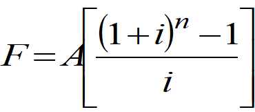
where A is an annuity, a constant dollar amount paid as an instalment each month. For an annuity of $1,000, a 36-month period and an interest rate of 10%/annum (0.0089%/month):

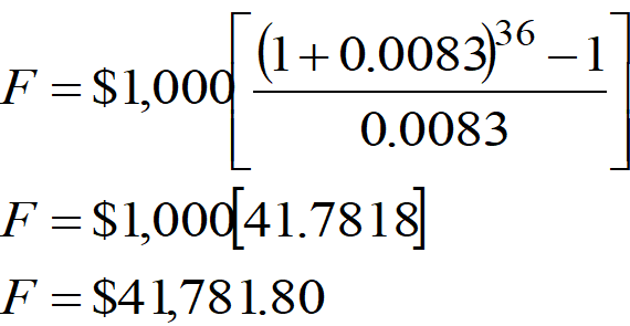
Each monthly instalment is added to the amount already in the account. Each month there is also a deposit made on the basis of how much money was in the account during the preceding month.

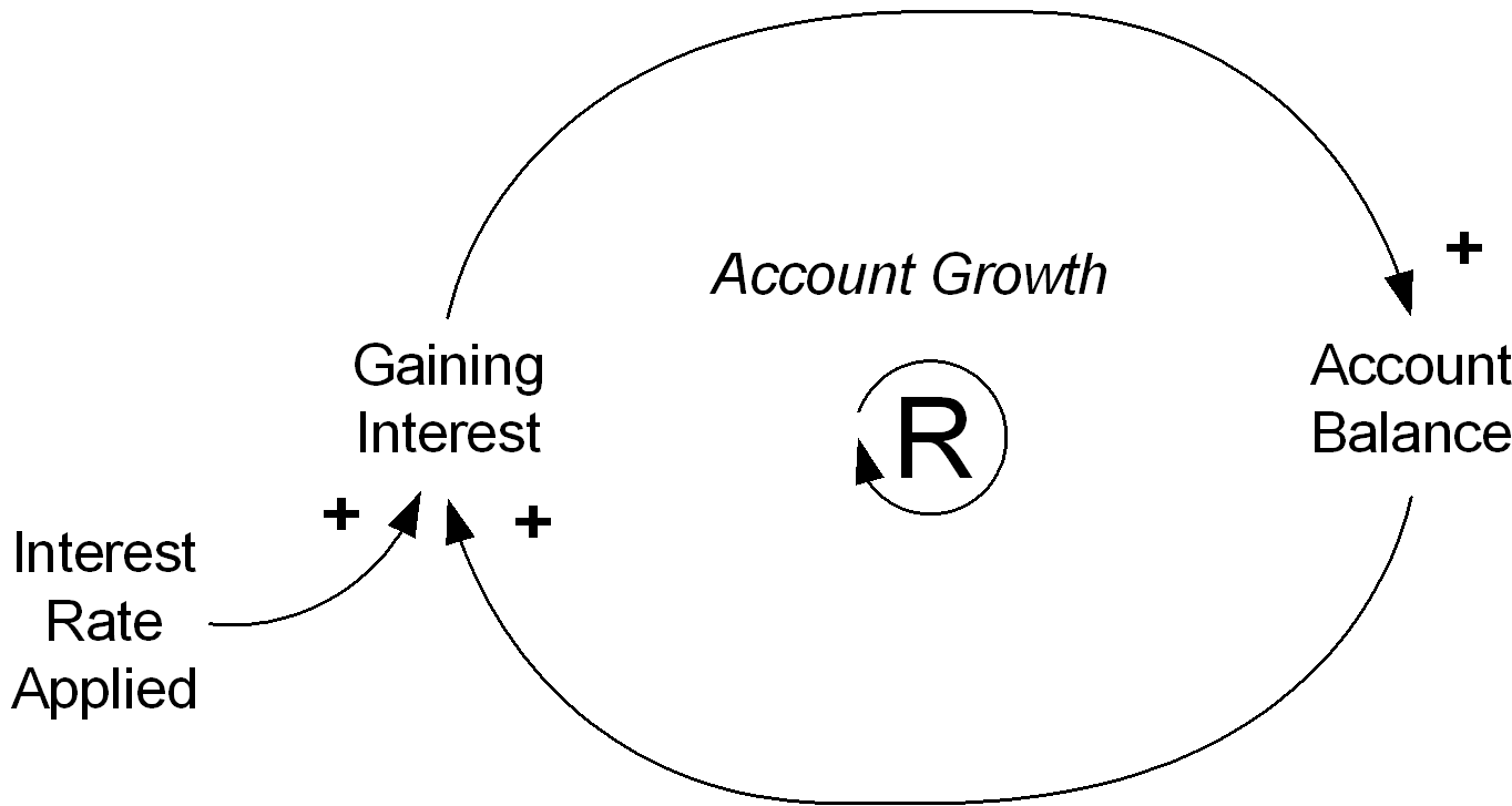
The compounding of interest based on the amount in the account and the rate of interest is a direct consequence of a feedback mechanism. Feedback involves taking the output and redirecting it as the input. In this instance the output, the current investment account balance, is multiplied by the interest rate per period, which, in turn, is then added to the account balance. This causes the account balance to grow at a rapid rate, which is most noticeable at the later stages of the investment period. Using systems thinking and system dynamics modelling conventions we can depict this as shown in Figures 1-10, 1-11, and 1-12.

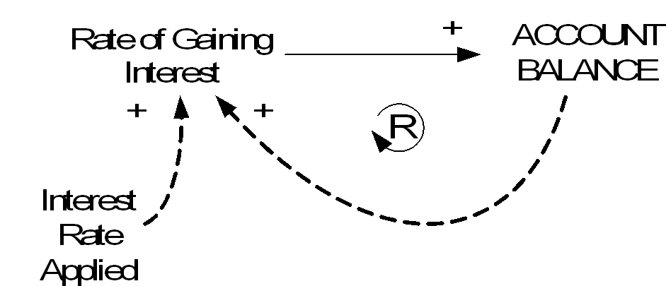
The causal depiction in Figure 1-10 follows the logic, that at any point in time, the size of the account balance causes interest to be gained and the larger the account balance the greater the amount of interest that will be added to the account balance. Note that ‘R’ inside a circular arrow denotes a positive (reinforcing feedback loop). The ‘+’ sign represents positive polarity of the link. Signs (‘+’ or ‘–‘) adjacent to the arrows are used to indicate polarity. A plus (+) sign implies that a change in the variable at the tail of the arrow causes a change in the variable at the head of the arrow in the same direction: a minus (–) sign implies that a change in the variable at the tail of the arrow causes a change in the variable at the head of the arrow in the opposite direction. Interest is calculated on the size of the account balance according to the prevailing interest rate.

The influence diagram, Figure 1-11 depicts the same information as the causal loop diagram but also shows ACCOUNT BALANCE, deliberately shown in upper case, as a state variable. The simplest way of thinking about a state variable is as a bathtub, that is, a device for accumulating stocks of items of interest, just as a bathtub holds water. If, for example, interest rate applied was set to zero, the rate of gaining interest would become zero, but the state variable ACCOUNT BALANCE would remain unchanged.

The stock-and-flow diagram of Figure 1-12 depicts exactly what the influence diagram does, but in this instance adds information about the initial balance of the account. The positive feedback loop is completed along the line of the physical flow from Rate of Gaining Interest to ACCOUNT BALANCE. Note that this is the direction of influence, from the influencing variable to the influenced variable. In the linear negative feedback example, which will be discussed later in more detail, the overriding

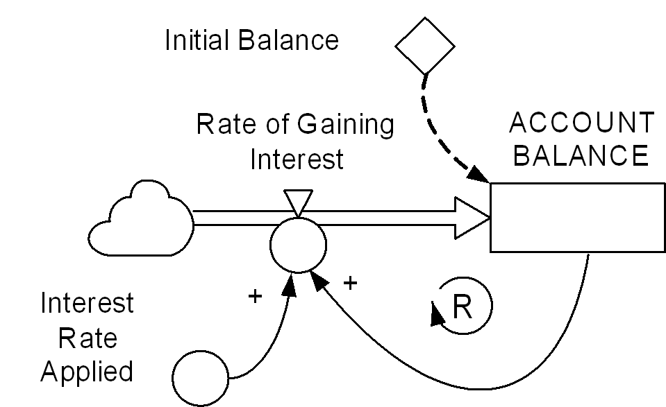
consideration remains that the direction of influence flow is from the influencing variable to the influenced variable, even though this runs counter to the physical flow

Consider an initial deposit of P₀. The shape of the resulting growth curve is characterised by the factor (1 + i )ⁿ, which operates on the current account balance. Actual growth appears as a series of increasingly larger steps at discrete periods of time (assuming no deposits, subsequent to the deposit made to open the account, are made). The balance at the end of each step is calculated using the formula, P_n = P_n-1 (1 + i )ⁿ. If the periods were to become infinitesimally short, and interest calculations are made for every one of these infinitesimally short periods, in effect, they are made continuously, the growth becomes exponential represented by P_t = P₀ e^it, where t is elapsed time. See Figure 1-13, where circles represent the end-of-period balances based on an initial deposit of P₀ to open the account, and no subsequent deposits.

There is considerable evidence to suggest that we seriously underestimate how these feedback structures operate and produce either growth as in this case, or decay, or work in combination to produce stabilizing behaviours.

References

- Rogers, M., 2001, Engineering Project Appraisal: The Evaluation of Alternate Development Schemes, Blackwell Science.