
A CAUSAL LOOP DIAGRAMMING CONVENTIONS
An essential part of system dynamics modelling is to make explicit what we have discovered about cause-and-effect underlying a problem situation. One way of making those causal hypotheses explicit is to draw causal loop diagrams. The prime purpose of creating any form of causal representation is to record dynamic hypotheses and communicate ideas during development of those hypotheses. This appendix briefly explains the conventions used in causal loop diagramming.
Conventions for depicting causal relationships have evolved over some 40 years of system dynamics modelling to the point where a relatively standard form exists. Causal loop diagrams and their uses are described in many texts and publications, including Roberts, et al. (1983), Roberts (1980), Goodman (1989), Senge (1990), Kim (various, especially in The Systems Thinker), Paich and Sterman (1993), Senge, et al. (1994), Richardson (1991; 1994; 1995; 1996; 1997) Maani and Cavana (2000).
The conventions used are described in detail by Sterman (1994; 2000: 137-190). In summary they are:
- Every link in your diagram, depicted as an arrow between variables, must represent what you believe to be causal relationships between variables. You must not include correlations between variables.
- Polarity should be indicated on every link in your diagram. Signs adjacent to the arrows are used to indicate polarity. A plus (+) sign implies that a change in the variable at the tail of the arrow causes a change in the variable at the head of the arrow in the same direction. Similarly, a minus (–) sign implies that a change in the variable at the tail of the arrow causes a change in the variable at the head of the arrow in the opposite direction.
- Each loop should be named with a very short title which represents the sense of the loop and has particular meaning to those involved in describing the problem or developing the causal loop diagram.
- Indicate important delays in causal links. Almost nothing happens instantaneously, so a case could be argued to indicate delay on every link. However, consider the time it takes for the delay in a particular link to produce an outcome and compare this with the time horizon applicable to the problem. If the delay is significant in relation to the time horizon, then indicate the delay. If, for example in Figure A-1, we are considering the impact of road congestion over a period of 3-5 years hence, and we know that major road upgrades typically take periods of six months or more, then the delay is significant. In the same example, one day or one week would not be significant.
- Variable names:
- should be nouns or noun phrases,
- must have a clear sense of direction, and
- should be chosen where normal sense of direction is positive.
- Layout is important for clarity:
- Use curved lines for information feedback. Curved lines also help the reader visualise the feedback loops.
- Make important loops follow circular or oval paths.
- Organise diagrams to minimise crossed lines.
- Do not use circles, hexagons or other symbols around variables—these only serve to add clutter and distract from the essence of the map.
- Be prepared to re-draw maps as many times as needed for clarity of ideas and understanding: modelling (both qualitative and quantitative) is iterative.
- Choose the right level of aggregation. This includes consistency in the level of aggregation across the whole of the map. Where greater detail (or lower level of aggregation) is represented in part of a map, then this suggests that either a separate map is needed for explaining the ideas contained there in or the detail should be set aside and summary statements of the variables and relationships are needed.
- Avoid creating large diagrams. Keep diagrams small, producing sets of interlinked maps on separate sheets of paper as needed.
- Make goals of negative loops explicit.
- Distinguish between actual and perceived conditions.
Figure A-1, which has been adapted from Sterman (2000:182) is an example of causal loop diagram drawn with consistency and level of aggregation in mind. It observes each of the diagramming conventions detailed above.
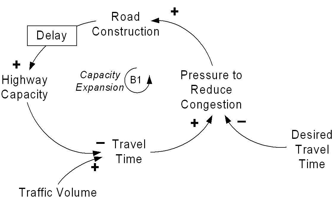
Reading directly from the map, it is easy to clearly and succinctly explain the problem. When drivers experience travel time increasing compared to the desired time to travel to their destinations, there is a resultant increase in pressure to reduce the congestion on the roads. This pressure translates through lobbying of local and federal government authorities to build more roads. Road construction increases highway capacity, but this does not occur immediately; building new highways or upgrading existing ones takes significant amounts of time. Increased highway capacity (without increases in traffic volume) reduces travel time. However, despite greater highway capacity, travel time could be increased by increasing traffic volume.
The Capacity Expansion loop is a balancing or negative feedback loop. This is first tested by working around the loop (starting at any point) and considering the effects of polarity on each causal link, ignoring (holding constant) the influences of any other causal links impacting from outside the loop under consideration or any delays encountered (delays do not impact on polarity). See Figure A-2.
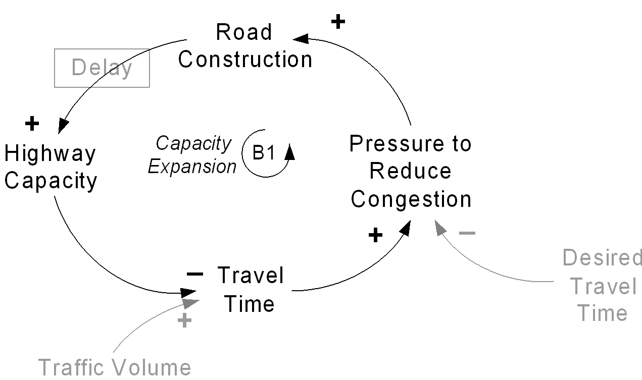
An increase in travel time will increase pressure to reduce congestion on the roads. In turn this increased pressure will produce increased road construction activity. Increased road construction activity leads to increased highway capacity. As highway capacity increases, travel time will reduce.
Conversely, as travel time decreases, pressure to reduce congestion on the roads will decrease and road construction start-ups will be less. Lower levels of road construction will mean less growth in highway capacity (indeed, there may be none—the situation may stagnate). With highway capacity decreasing through lack of road works (particularly maintenance of existing roads), travel time will increase.
To confirm that this is a negative feedback loop, count the number of negative polarity signs around the loop. In this instance it is one, which is an odd number. An odd number of negative polarity signs gives us and indication that the feedback loop is negative, or balancing. Zero or an even number or negative signs would indicate a positive feedback, or reinforcing loop.
References
- Roberts, N.R., Andersen, D.F., Deal, R.M., Garet, M.S. and Shafer, W.A., 1983, Introduction to Computer Simulation: The System Dynamics Approach, Productivity Press, Portland Oregon.
- Roberts, E.B., 1980, Managerial Applications of System Dynamics, The MIT Press, Cambridge, Massachusetts.
- Goodman, M.R., 1989, Study Notes in System Dynamics, Productivity Press, Portland, Oregon.
- Senge, P., 1990, The Fifth Discipline: The Art And Practice Of The Learning Organisation, Doubleday, New York.
- Paich, M. and Sterman, J.D., 1993, “Boom, bust, and failures to learn in experimental markets”, in Management Science, Vol. 39, No.12: 1439-1458.
- Senge, P., Roberts, C., Ross, P.B., Smith, B.J. and Kleiner, A., 1994, The Fifth Discipline Field Book: Strategies and Tools for Building a Learning Organisation, Nicholas Brealey Publishing, London.
- Richardson. G.P., 1991, Feedback Thought in Social Science and Systems Theory, University of Pennsylvania Press, Philadelphia.
- Maani, K.E. and Cavana, R.Y., 2000, Systems Thinking and Modelling: Understanding Change and Complexity, Prentice Hall.
- Sterman, J.D., 1994, “Learning in and about complex systems”, in: System Dynamics Review, Vol. 10, No. 2-3, (Summer-Fall): 291-330.
- Sterman, J.D., 2000, Business Dynamics: Systems Thinking and Modelling for a Complex World, Irwin McGraw-Hill.