
6.4.7 Assuring Integrity Of Units Used In Models
Regardless of how tempting and expeditious it might seem to build models without assigning units, dimensionless models should never be constructed. Powersim™ Studio has been designed to assure the assignment of units at every stage of construction. Even for an experienced modeller, it may not be clear exactly what units are to be assigned at a particular stage of construction. However, it is always possible to determine what units should be used. In most instances, Powersim™ Studio will help at least by indicating when you do not have the units correctly assigned.
Key considerations are:
- Conversion of units from one form to another is easily achieved by multiplying the quantity and its units by unity. We can do this as often as we need without changing the original quantity. This method ensures the integrity of units used. This is demonstrated below.
- Each time we encounter, or insert, a rate variable into the physical flow of a model, the appropriate units will be those of the stock (level or accumulator) into which or out of which the flow occurs, but these are divided by time. This is because the insertion of each of the rate variables results in mathematical integration being performed.
Conversion of Units by Unity Multiplication
Example: Calculate the equivalent in litres per 100 kilometres of 20 miles per (imperial) gallon.
The first step involves arranging the quantity and the units you need to convert into the form required. Here we have miles per gallon and we want litres per kilometre. We will convert litres per kilometre to litres per 100 kilometre at a subsequent stage.
The form of answer we want is litres / kilometre. This is volume divided by distance, whilst we are starting with miles per gallon which is in the inverse form. Before we can commence we must rewrite 20 miles per gallon in the form:
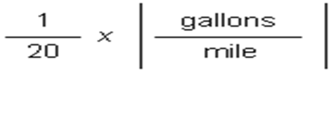
The strategy is to multiply each stage by unity. This is achieved by ensuring that the numerator (above the line) and denominator (below the line) are exactly the same, resulting in the quantity between the vertical lines always being equivalent to 1, that is, unity.
A sufficiently accurate rule of thumb for the relationship between imperial gallons and litres is that 200 litres = 44 gallons. Alternatively, the conversion factor 4.546 litres per 1 imperial gallon might be used.
Similarly, a sufficiently accurate rule of thumb for the relationship between kilometres and miles is that 8 kilometres is approximately equivalent to 5 miles. Alternatively, the conversion factor of 0.62137 kilometres per 1 mile might be used.
Using our rules of thumb conversions to multiply the original quantity and units by unity, yields the progressive development of our overall conversion.
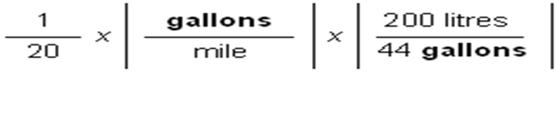
Note that the first unity multiplication involves converting gallons to the required units of litres: gallons appear in bold and units in opposing positions above and below the line cancel each other out. We follow this theme to convert miles to kilometres.

Further, we must multiply by 100 to complete our conversion, noting that for our units to be correct we must be able to travel 100 kilometres: we multiply by 100:

We can now rule a line through units which appear both as numerator and denominator:

Our numerical answer is calculated as:

Our numerical answer is:
14.20 litres per 100 kilometres
Mathematical Integration Introduced by Successive Linking of Stocks to Rate Variables
Rate variables control flows, and flows are expressed as flow units per unit of time. Consider the example at Figure 6-1, where:
- a flow rate of items per second (items/s) is needed to produce accumulation in a stock of ITEMS (items), and
- a flow rate of items per second per second (items/s/s) is needed to produce accumulation in a stock of items per second (items/s).
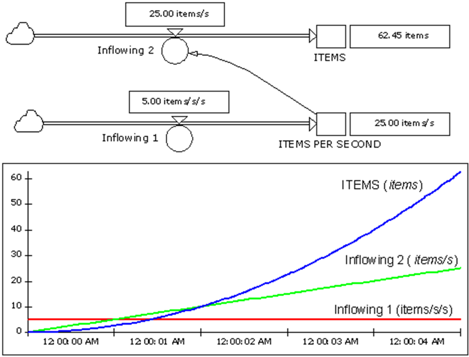
The accumulation is produced by that form of mathematical addition over each incremental element dt of time which we know as integration, through which we calculate the incremental increase or decrease in the area under a curve:
- calculating the incremental change area under the Inflowing 1 curve (a straight line, indicating equal-sized increments) added in any timestep gives us constant incremental increases in the downstream stock, ITEMS PER SECOND, which is a straight line shown as linked rate variable Inflowing 2; and
- calculating the area under the Inflowing 2 curve (graph) added in any timestep (which increase in size each subsequent timestep) gives us the incremental increase in the downstream stock, ITEMS, which appears as the graph of a quadratic expression.
The results of arithmetic integration are:
- an arithmetic constant returns a linear algebraic function, and
- a linear algebraic function is a quadratic algebraic function.
Each time arithmetic integration is performed, the power of the variable being integrated is raised by one. Where integration is performed with respect to time, as is the case in time-domain modelling, such as system dynamics modelling is, the terms of the expression involving time are raised to the next higher power. This must be accompanied by a change in the units as indicted in Figure 6-1, from items/s/s for Inflowing 1 to items/s for Inflowing 2, to items for ITEMS.