
F.6 MODULE—FIRST ORDER LINEAR NEGATIVE FEEDBACK
F.6.1 General Description
The first-order negative feedback module comprises a stock progressively depleted at a rate dependent upon a fractional decay factor. At any time, the absolute value of the decay is indicted by the content of the stock. More correctly, the initial sate will be depleted over time to become the current state—the extent of the decay can be gauged by counting all that flows out over the period of interest. Rate of change of state is:
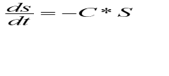
where:
C = a constant, and
S = state of the system
A first-order negative feedback has the effect (each time we calculate it) of subtracting from S an amount (where the constant is a Fractional Decay Factor ‘d’) which is less than the previous time we calculated it. Consider a series of calculations at times t0, t1, t2 … tn, with the initial value of S being S0 and a Fractional Decay Factor d operating on the outflow. The state of the system will change as shown in Table 6-1.
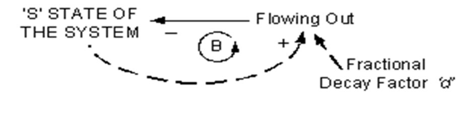
The negative (balancing) feedback loop has the effect of depleting the stock through the net outflow rate, that is, the net change of state calculated at each time-step.
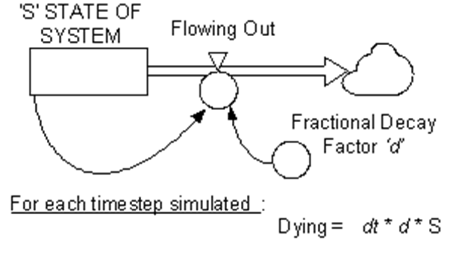
Table F6-1. Change of State with Time—First-order Linear Negative Feedback
tn | Current State ‘S’ | Net Change of State |
|---|---|---|
0 | S0 | 0 |
1 | S 1 = S0 – d * S0 | – d* S0 |
2 | S2 = S0 – d*( S0 – d* S0 ) S2 = S0 – d*( S 1 ) | – d*( S 1 ) |
3 | S3 = S0 – d* (S0 – d*( S0 – g* S0 ) ) S3 = S0 – d*( S 2 ) | – d*( S 2 ) |
… | ||
n | Sn = S0 – d*( S n-1 ) | – d*( S n-1 ) |
F.6.2 Reference Sources
The module is described here after Goodman (1989: 35-48), Sterman (2000: 275). Further explanation of this module can be found at Sterman (2000: 275).
F.6.3 Module Influence Diagram
The influence diagram for this module is shown in Figure F6-2.
F.6.4 Application
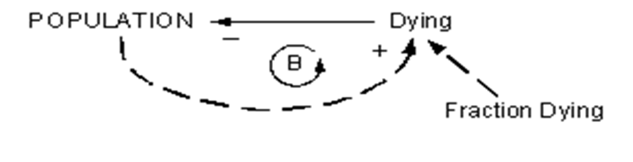
An example would be the decay of radioactivity of a fixed (initial) quantity of a radioactive isotope. Decay of a population through deaths as people age, where a fraction of the remaining population dies each year, involves a similar mechanism.
F.6.5 Causal Diagram Representations
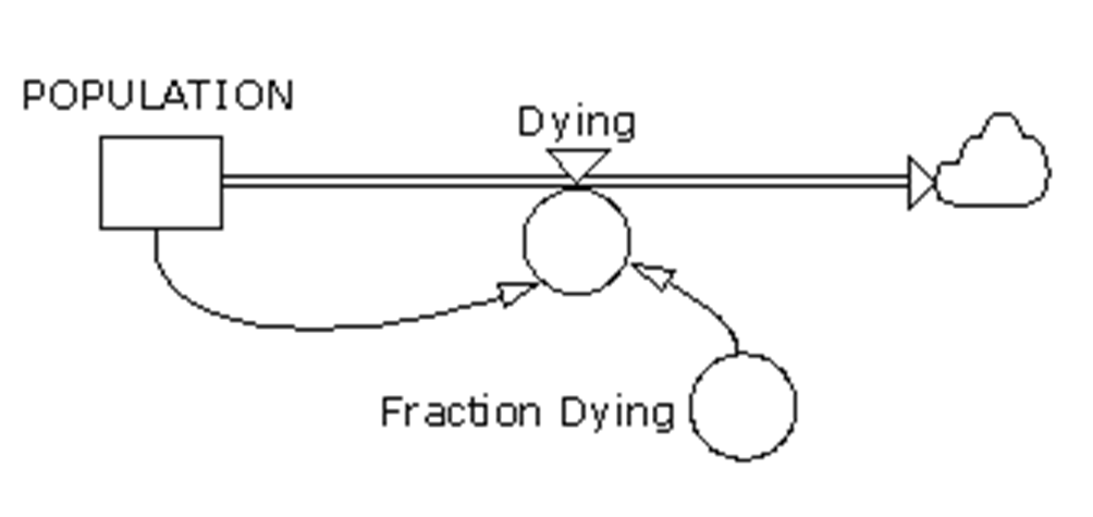
The influence diagram would be as shown in Figure F6-3. The equivalent stock-and-flow diagram would be as shown in Figure F6-4.
F.6.6 Functional Description
The functions of the various parts of the module are described in Table F6-2.
Table F6-2. Functional Description—First-order Linear Negative Feedback Module—POPULATION Example
Variable | Function | Comment |
|---|---|---|
Fraction Dying | 5% | This is the fraction of the population dying at any point in time, expressed as a percentage. Units are expressed as, for example, <<% pers / yr>>. If this fraction were to remain unchanged during the simulation, it would be defined as a constant with the more appropriate diamond icon. |
Dying | POPULATION * Fraction Dying | In this module, Dying is subtracted in increments via the flow valve controlled by the auxiliary variable Dying. Dying will subtract incremental amounts (each timestep) equal to POPULATION*Fraction Dying. Units: <<pers/time>> |
Initial Population | 55,750 | The initial population is defined within the POPULATION variable. Units: <<pers>>. |
References
- Goodman, M.R., 1989, Study Notes in System Dynamics, Productivity Press, Portland, Oregon.
- Sterman, J.D., 2000, Business Dynamics: Systems Thinking and Modelling for a Complex World, Irwin McGraw-Hill.