6.4.9 Extreme-Value Testing
Extreme-value tests are designed to investigate the response of the module or model to extreme-value inputs. Every module, sector, or model we create must be able to cope with input values even well outside likely to be experienced under normal conditions. Extreme-value tests should always produce logical results, even though the inputs are unlikely to be encountered in practice.
Conducting extreme-value tests is an essential part of verifying that a model will perform as intended. Functional performance of the model must be tested under a wide variety of conditions, including the most extreme ones. We need to design and apply extreme-value tests even though we might not imagine easily how the extreme circumstances represented by each specific test might arise in practice. By providing inputs that are extreme, such as very small or zero, large in either a negative or positive sense, or that step from being negative or positive we apply stress to the model. Such tests will reveal whether or not the model can cope with input values outside the narrow ranges for which we might have originally designed the model.
Extreme-value tests are also valuable in helping to identify potential instability in model behaviour. Applying sharp disturbances or strong impulses to values of input variables should not result in the model becoming unstable or oscillating for long periods.
It is not only our models that behave in unexpected or undesirable ways as a result of inputs which produce instability. A famous example of how disturbances can cause vibration and instability in large engineering structures is that of the collapse of the Tacoma Narrows Bridge. Situated on the Tacoma Narrows in Puget Sound, near the city of Tacoma, Washington, in the United States, the bridge had only been open to traffic for a few months. On the morning of 7th November, 1940, after several days of steady winds blowing through the Tacoma Narrows, steadily-increasing amplitudes of vibration were produced. The suspension bridge across the Narrows finally began to resonate with amplitudes of vibration of several metres. These violent vibrations caused the bridge to collapse in the most dramatic way.
There are exceptions where this type of behaviour is not a concern, but these will be problems where dynamic instability or long-lived transient effects or resonance is a known characteristic and, therefore, is expected to occur. Step changes in input values are particularly useful for testing stability.
Caution is needed when we design extreme value tests. We cannot simply change the values of selected parameters to extreme ones without analysing first what the effects of those changes might be. Extreme value tests need to be specified in two parts:
- the test to be applied, and
- model response expected.
Of course the latter cannot be determined in advance if detailed functioning of the model is not clearly understood. Consequently, such tests are valuable not only to test the model but to test the modeller’s understanding of the detailed functioning of that model.
Example—Implications of Extreme-Value Test Design
In the double pendulum problem, we might be tempted to test the model’s capacity to behave as a simple pendulum by effectively removing the second suspended mass m2. To do this we might choose a strategy of simultaneously setting both m2 and l2 to zero in the following expression for angular acceleration for the pendulum B-C:

If we attempt to set both m2 and l2 to zero, this will produce a denominator of zero: this is problematic because we cannot divide by zero. In practice, we can set only m2 to zero, giving the equation, which should return zero for all expected values of the variables in the numerator:
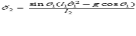
For the right hand side of this expression to be effectively zero, l2 must be set to a very large value: in effect l2 must become infinitely large. This might mean setting l2 at a value of 100,000 metres or larger (noting that we have already set m2 to zero). Then, for practical values of variables in the numerator, angular acceleration effectively becomes zero.
The expression for angular acceleration of pendulum A-B is:

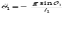
Noting that m2 = 0, this expression becomes the correct expression for angular acceleration of a simple pendulum: