3.1.6 Flowing In Powersim™ Studio Module

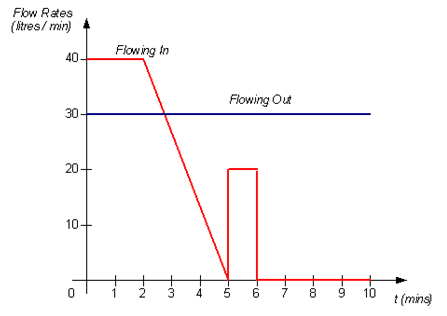
The basic requirements for a module we will design to analyse Flowing In can be derived from Figures 3-16, 3-17, and 3-18. These are shown in Figures 3-19, 3-20, and 3-21.

Figure 3-16. Influence Diagram—Flows Affecting *BATHTUB*

Figure 3-17. Stock-and-Flow Diagram Flows Affecting *BATHTUB*

Figure 3-18. *Flowing In* and *Flowing Out* Rated Defined

Figure 3-19. Influence Diagram—*Flowing In* Module

Figure 3-20. Stock-and-Flow Diagram—*Flowing In* Module

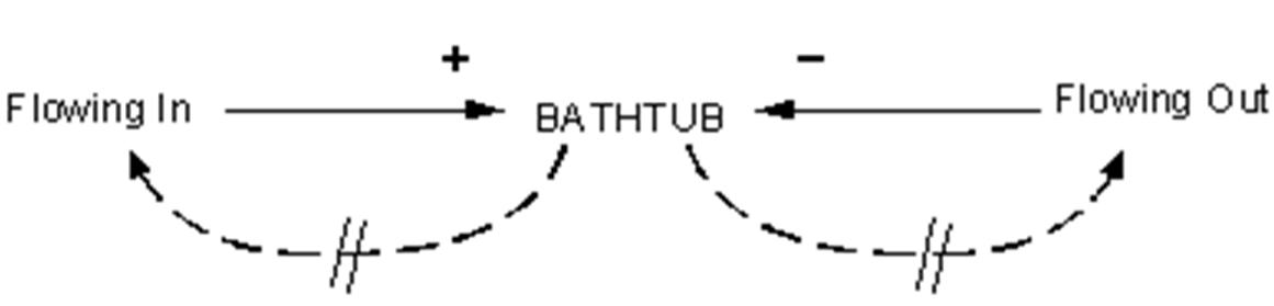
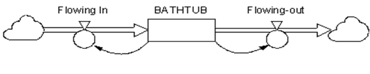
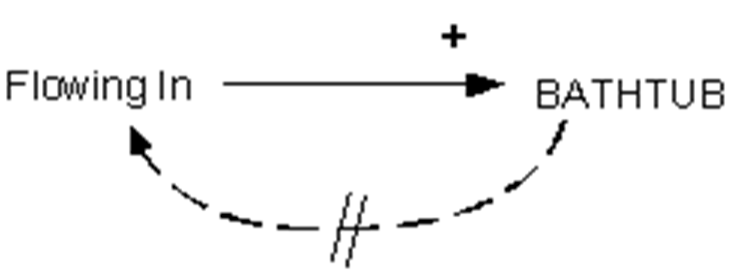
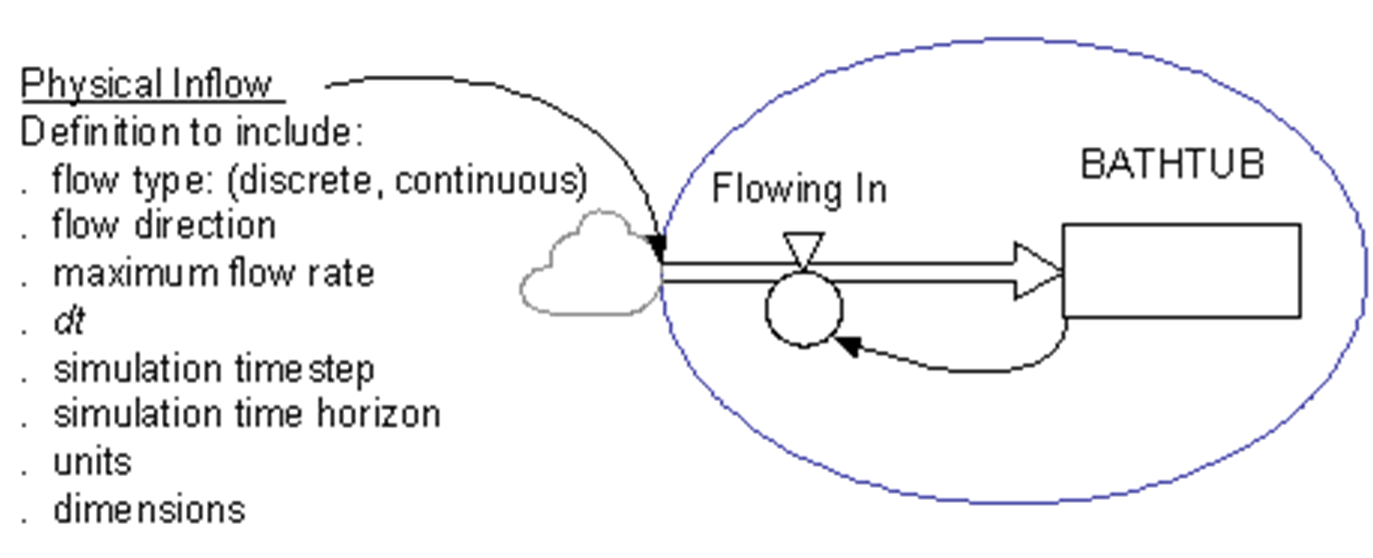
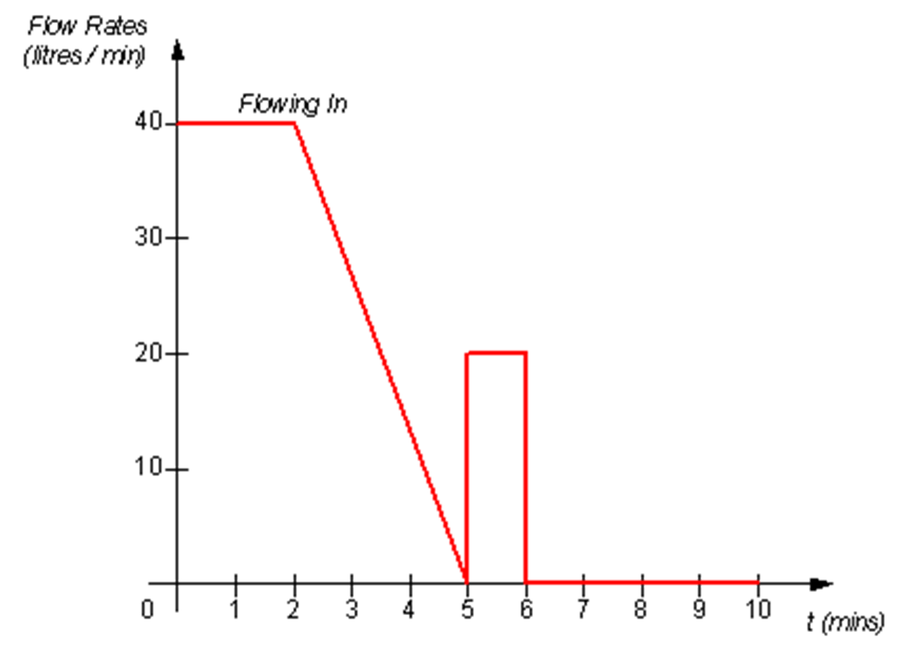
In addition, the following governing business rules are to be included in the model:

Initial contents of BATHTUB amount to 40 litres.
The simulation is to be paused and inflow is to stop at 298 litres just before BATHTUB becomes full. This assumes the maximum capacity is 300 litres.

The module is defined in Table 3-2.

Table 3-2. Definition of Flowing In Module

Variable	Variable Type	Units	Definition
Flowing In	Rate variable. Continuous physical flow. Material flowing is water.	litres / minute	Flow from outside boundary into module. Maximum flow rate = 40 litres / minute. Figure 21 shows rate of Flowing In. Simulation starts at t = 0 and runs until t = 10.
BATHTUB	State variable.	litres	Stock of water. Initial value is 40 litres. Maximum = 298 litres.

Variable

Variable Type

Units

Definition

Flowing In

Rate variable.

Continuous physical flow.

Material flowing is water.

litres / minute

Flow from outside boundary into module.

Maximum flow rate = 40 litres / minute.

Figure 21 shows rate of Flowing In.

Simulation starts at t = 0 and runs until t = 10.

BATHTUB

State variable.

litres

Stock of water. Initial value is 40 litres. Maximum = 298 litres.

Project and Simulation Settings. The project and simulation settings needed for the creation of this module and running of the simulation are:

Project Settings. Main elements of project information are:
<Project>
<Project Settings>
<Time Measurement>
<Available Calendars>, select:
<Gregorian> (although selection of type of calendar is of little consequence in this simulation).
<Time has unit>, select:
<Minute> (Note that it is recommended that the option ‘Time has unit’ always be selected as ‘Yes’).
Simulation Settings. Simulation setup settings are:
<Simulation and Settings>
<Simulation>
<Time Settings>
<Calendar> :
<Gregorian>
<Timestep>—select:
00:00:00.05, that is, 0.05 seconds (Timestep of 0.2 seconds or less would be appropriate to return required accuracy—much smaller Timestep values would demand increased computation and would slow simulation runs);
<Start Time>—select:
1/01/2005
<Stop Time>—select:
1/01/2005 0:10:00
<Integration>—select 1^st Order Euler (fixed step) integration. Note that there are two points in Flowing In were values change very rapidly and this will impact on the extent of the error associated with the numerical method which approximates mathematical integration. Alternatively we might choose, 2^nd Order Runge-Kutta (fixed step) integration and compare the resultant variation in BATHTUB over the simulation run. Here we know that the precise answer is 200 litres, and that knowledge should be used to inform choices of ‘Timestep’ and ‘Integration’.
Create Units. There is a need to add units of litres (Note that metres are automatically added by Powersim™ Studio. This is because the units of litre (volume) and metre (length) are connected by the fundamental relationship; 1 litre = 0.1 metre * 0.1 metre * 0.1 metre):
<Project>:
<Global Units>—add ‘Standard Unit’ <<Liter>> (Note that Powersim™ Studio uses the spelling ‘Liter’ and ‘Meter’ respectively).

The Flowing In module developed in Powersim™ Studio is described below. The constructor diagram with auto reports displayed at the end of the 10-minute simulation is shown at Figure 3-22.

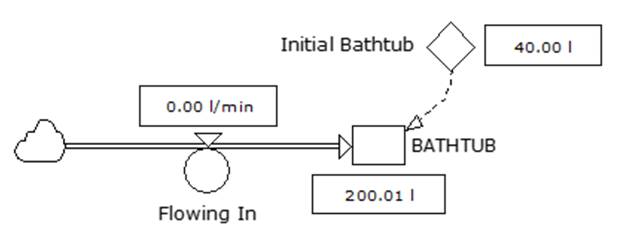
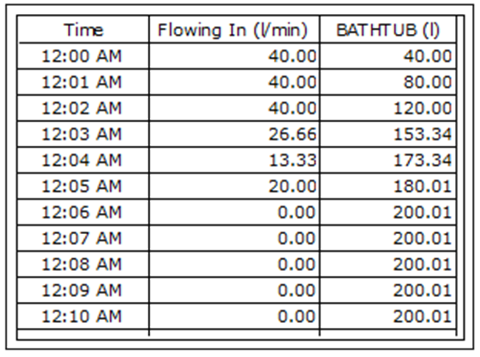
Figure 3-22. The Powersim™ *Studio* *Flowing In* Module Showing Auto Reports at *t = 10* mins

Note that the value of BATHTUB at the end of the simulation is 200.01 litres rather than exactly 200 litres. This is a consequence of the numerical method used by Powersim™ Studio to calculate incremental area under the Flowing In curve. Note that all such software applications use numerical methods which, of necessity, give approximate answers. By careful model design and choice of simulation settings, the errors associated with such approximations can be kept sufficiently small to be insignificant.

The error can be reduced by a combination of reducing the size of dt (set as ‘Timestep’ in ‘Simulation Settings’ dialogue box in Powersim™ Studio) or by choosing a higher order of integration used (set as ‘Integration Order’ in ‘Simulation Settings’ dialogue box in Powersim™ Studio). Simply put, the higher the order of integration employed the greater will be the capacity of the numerical (approximation) method to cope with rapid changes in slope, or variations in the value, of the time-dependent variable being integrated.

However, selecting smaller values of dt and higher orders of integration will demand greater numbers of computations and will slow down the simulation. This can be important when simulating models which involve large numbers of integrations (as indicated by the numbers of rate-controlling variables and feedback loops in the model).

The algebraic formulation of Flowing In is shown at Figure 3-23.

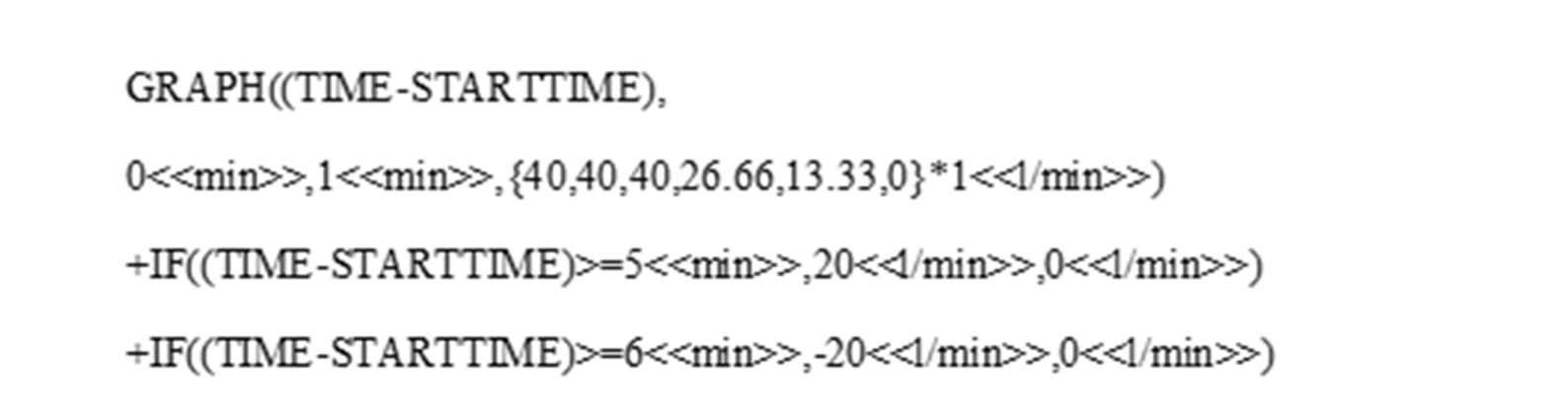
Figure 3-23. Formulation of Definition of *Flowing In* Rate-Controlling Variable

Note that this formulation combines Powersim™ Studio’s ‘GRAPH’ function and two ‘IF’ functions. The latter are effectively used as ‘STEP’ functions (the ‘STEP’ function may have been used as an alternative). This is necessary because the ‘GRAPH’ function allows for changes in values each ‘TIMESTEP’ but does not readily accommodate a dramatic change in value of the plotted variable.

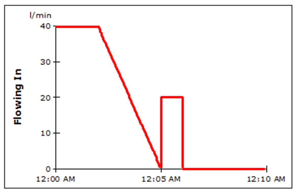
Flowing In changes from a zero litres / minute at t = 5 minutes to 20 litres / minute an instant later. An alternative method might involve using a much smaller dt, typically a second. This would prove to be impractical because it would demand specifying every data point on the graph, that is, for each second over the 10-minute simulation.

The results of defining Flowing In as described at Figure 3-23 are shown at Figure 3-24.

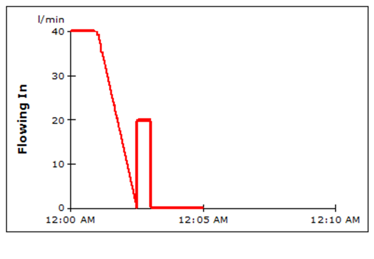
Figure 3-24. Graphical of Definition of *Flowing In* Rate-Controlling Variable

Caution When Using TIMESTEP Function. In a number of examples in the Powersim™ Studio Reference Guide it is suggested that (TIME-STARTTIME)/TIMESTEP be used in instances such as formulating the definition of rate-controlling variables. If this is done, there is need for caution: the TIMESTEP cannot be changed without changing the variable.

Consider, for example, Figure 3-24. If (TIME-STARTTIME) in Figure 3-23 were replaced by (TIME-STARTTIME)/TIMESTEP and the TIMESTEP subsequently halved, the graph would be compressed to a simulation of five minutes rather than 10 minutes, as shown in Figure 3-25. This can be problematic since we routinely change TIMESTEP during model testing and verification.

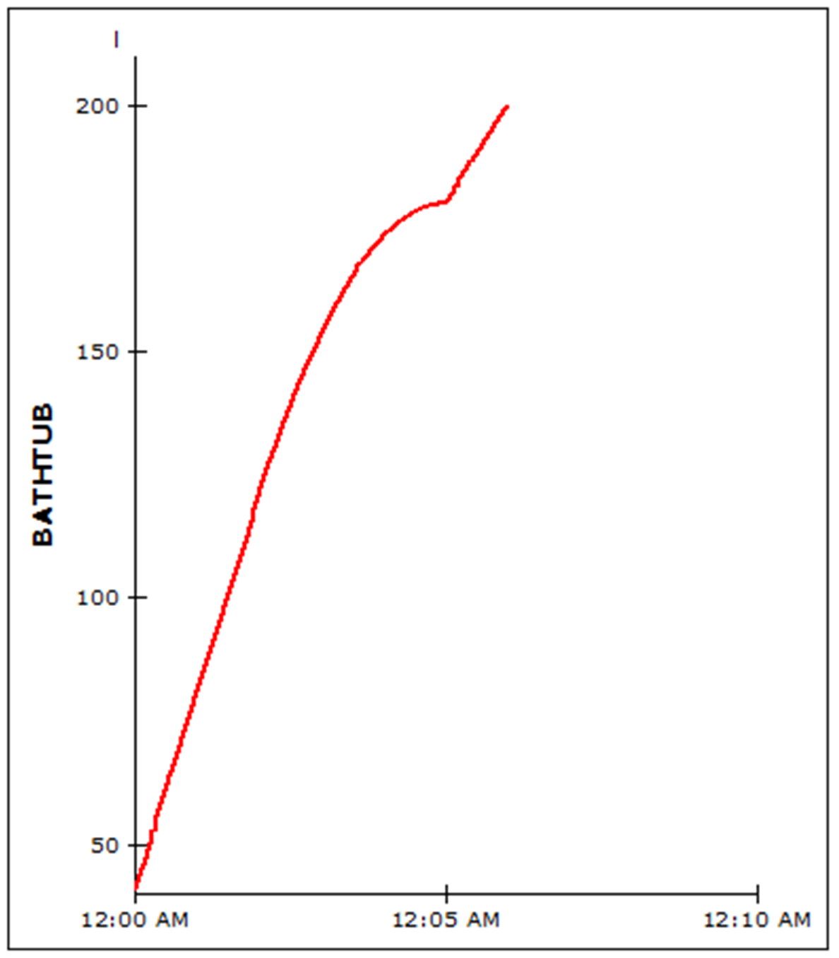
Figure 3-25. Effect of Reducing dt by Half Where ((TIME-STARTTIME)/TIMESTEP) is Used

The Time Table printout for each minute of the simulation, showing Flowing In and BATHTUB is in Figure 3-26.

Figure 3-26. Time Table Printout of *Flowing In* and *BATHTUB*

The time graph for BATHTUB is shown in Figure 3-27. We expect that Figures 3-26 and 3-27 represent values identical to Figure 3-13, although a very small error is evident in the Powersim™ Studio simulation. Note that the simulation stops at 6 minutes and 40 seconds.