Decision Making / 6 / 6.9 / 6.9.2

6.9.2 Developing And Interpreting The Causal Loop Diagrams For Threetwoone’s Problems

Causal loop diagrams are becoming increasingly common in business. Sterman (2000: 137-190) provides an excellent explanation of how to build, read and interpret casual loop diagrams. The essentials are summarised in this section.

Causal loop diagrams provide a ‘quick and dirty’ way of capturing the hypotheses about the causes of the dynamics of the focal problem. Causal loop diagrams can be used as we have used cognitive/concept mapping to support the processes of knowledge elicitation and capturing of mental models of individuals or teams, but at a level of aggregation higher than that for cognitive/concept mapping. Causal loop diagrams have been found to be excellent aids in communicating and summarising the important feedback loops responsible for a particular problem: causal loop diagramming works particularly well in group modelling situations.

Contemporary conventions for causal loop diagramming are the product of over 30 years development. These conventions are relatively simple but must be followed faithfully. Idiosyncratic symbols and styles must be avoided as they make causal loop diagram confusing to read and understand.

There are many similarities in the conventions of cognitive/concept mapping and causal loop diagramming. There are also several key differences. Where they exist, they will be explained as we proceed through the process of building a set of causal loop diagrams depicting ThreeTwoOne’s problems.

Unlike cognitive/concept maps which deal with concepts or schemata, causal loop diagrams deal with variables. A variable is a measurable quantity used to describe the state of the system under investigation. In dynamic problems, variables are continually changing. For example, temperature is a variable used to describe how hot or cold a room is. We would use temperature (ºC) as a state variable in description of the operation of the air conditioning system in a building or home. In causal loop diagramming, variables are linked by causal arrows only: connotative and conflict links used in cognitive/concept mapping are not used in causal loop diagrams. Figure 6-8 shows basic causal loop diagramming conventions.

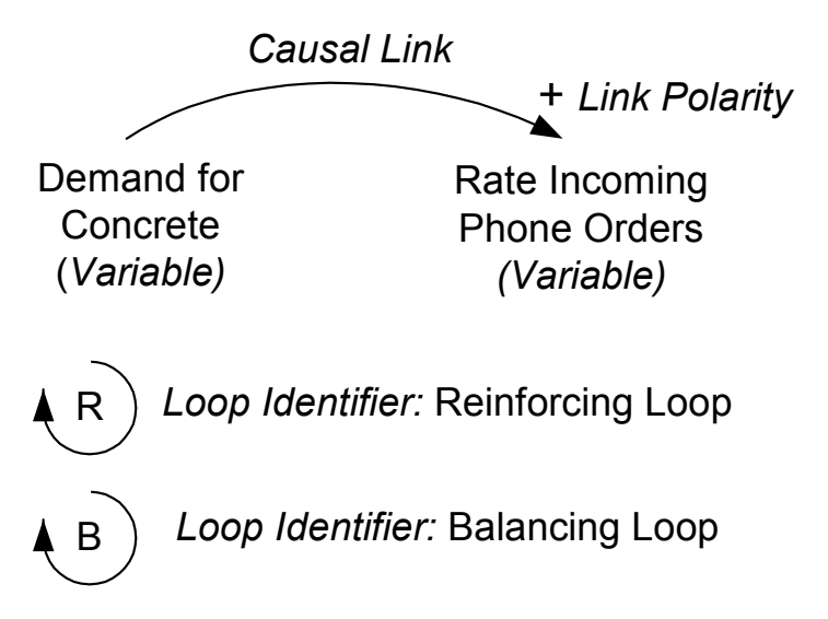
Here, Demand for Concrete (a variable) creates or causes the generation of Incoming Phone Orders (a variable) at a particular rate. In this example, link polarity is positive: as demand increase the rate of incoming phone orders increases and a decrease in demand produces or causes a decrease in incoming phone orders. Where linked variables produce a feedback loop, the loop can be either reinforcing or balancing as explained below.

Important feedback loops are identified in causal loop diagrams we build. Figure 6-9 contains an example.

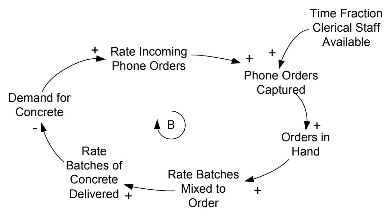
Figure 6-9 shows that as demand for concrete increases, the rate at which incoming orders is received also increases. This assumes that there are a number of customers each with relatively small, similar sized orders. The number of orders captured is dependent upon the fraction of time that the clerical staff members are available to attend to the telephone. Orders captured are logged and passed to the batching plant. Depending on a range of factors not yet included in the diagram, such as batch plant capacity, the batches are mixed to order. The rate of mixing determines the rate at which deliveries can be made and demand for concrete satisfied. As deliveries occur, demand for concrete is satisfied. The polarity of this last causal link is negative, that is, as the rate of delivery goes up demand is satisfied and demand goes down. By the same argument if the rate of delivery of batches of concrete decreased, there would be an increasing level of unsatisfied demand for concrete. The fastest and easiest way to determine whether a particular loop is reinforcing (positive) or balancing (negative) is to add up the negative signs around the loop. If there are none or the number is even, then the loop is a reinforcing (positive) one. Where the number of negative signs is odd, the loop is balancing (negative).

The correct way of determining the polarity of a feedback loop is to start at a particular point, say, at Demand for Concrete node and imagine a small change at that node and trace the effects of that change around the loop. If the feedback effect reinforces the original change, the loop is positive; if it produces a change in the opposite direction, it is a negative loop.

In its present form, the diagram does not account for any delays in the processes. It should be intuitively obvious that there are a series of delays in activities such as answering the telephone, logging orders, mixing concrete, loading trucks, driving to site and delivering.

In a causal loop diagram all links should have unambiguous polarity. If polarity is not indicated, by default it is assumed to be positive. However, for clarity and completeness, polarity of each link and each loop should be indicated by at ‘+’ or ‘-’ sign.

In cognitive/concept mapping, we can have situations where a link can be either positive or negative or the causal effect may even working the opposite direction under certain conditions. This, of course, is the connotative link. The conflict link is a special case of the connotative link where there is a state of stress or disharmony between the nodes at the ends of the link. This cannot exist in casual loop diagramming where causality must operate clearly and unambiguously and only in one direction. For this reason, we cannot have double-headed arrows or pairs of arrows acting in opposite directions in causal loop diagrams. Remember that in cognitive /concept mapping we use a connotative link to represent situations where we might be tempted to draw a double-headed arrow or pair of arrows acting in opposite directions.

In causal loop diagramming, if you feel the need to draw double-headed arrows or pairs of arrows acting in opposite directions, this generally means there is a need to insert a missing node (variable). Inserting the missing variable should help make the direction and polarity of the causality completely clear.

In Figure 6-9, there are two casual inputs to Phone Orders Captured. This is because the number of phone orders captured is dependent on more than just Rate of Incoming Phone Orders. In reality, clerical staff must attend the telephone: if the office is unattended and a potential customer phones, this order is likely to be lost. If the Time Fraction Clerical Staff Available was 100% then all incoming phone orders should be captured. This assumes, of course, that all calls are very short.

To make subsequent discussion about any causal loop diagram easier, it is necessary to give each important feedback loop a number and a name. We have already indicated in Figure 6-9 that the loop is a balancing one. Noting this is the first balancing loop we have drawn, we might label it ‘B1’ and name it ‘Demand Through to Delivery’. A more complete casual loop diagram representing the capturing of orders, production and satisfying customer demands might be as shown at Figure 6-10.

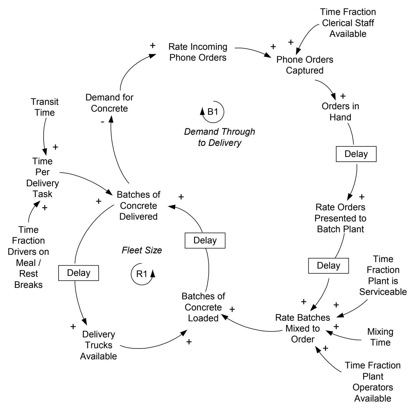
Whilst we might draw other casual loop diagrams, say, to depict operating and capital costs and incorporate them into the diagram at Figure 6-10, we need to consider what those diagrams might add. The aim is to identify where risks are and where best to direct our management intervention and assign resources. Figure 6-10 provides insights that immediately allow the formulation of intervention strategies. These identified by working systematically around the casual loop diagram. What this can reveal is explained at Section 6.9.4.

References

- Sterman, J.D., 2000, Business dynamics: Systems thinking and modelling for a complex world, Irwin McGraw-Hill.