6.4.3 Frequency Spectrum Of An FM Wave

Equation (6.25) can be rewritten in terms of m_f and angular frequencies:

υ (t) = V_{c} \cos (ω_{c} t + m_{f} \sin ω_{m} t)

(6.29)

This can be further expressed as a sum of sinusoids by firstly expanding:

υ (t) = V_{c} [\cos ω_{c} t \cos (m_{f} \sin ω_{m} t) - \sin ω_{c} t \sin (m_{f} \sin ω_{m} t)]

(6.30)

and then noting the trigonometric relationship that:

\cos (m_{f} \sin ω_{m} t) = J_{0} (m_{f}) + \sum_{n e v e n}^{\infty} 2 J_{n} (m_{f}) \cos (n ω_{m} t)

(6.31)

\sin (m_{f} \sin ω_{m} t) = 2 \sum_{n o d d}^{\infty} J_{n} (m_{f}) \sin (n ω_{m} t)

(6.32)

where J_n(m_f) are Bessel functions of the first kind, of order n and argument m_f.

Substituting Equations (6.31) and (6.32) into Equation (6.30) and expanding products of sines and cosines finally results in:

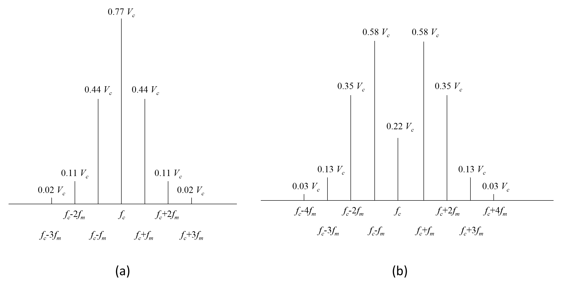
υ (t) = V_{c} J_{o} (m_{f}) \cos ω_{c} t + \sum_{n odd}^{\infty} {V_{c} J}_{n} (m_{f}) [\cos (ω_{c} + n ω_{m}) t - \cos t (ω_{c} - n ω_{m})] + \sum_{n even}^{\infty} {V_{c} J}_{n} (m_{f}) [\cos (ω_{c} + n ω_{m}) t + \cos t (ω_{c} - n ω_{m})]

(6.33)

which provides a mathematical expression of a wave whose amplitude is constant and whose instantaneous frequency is varying sinusoidally. The amplitudes of the sidefrequencies and carrier depend on the value of the modulation index, as described in Equation (6.33) and shown in Figure 6.18.

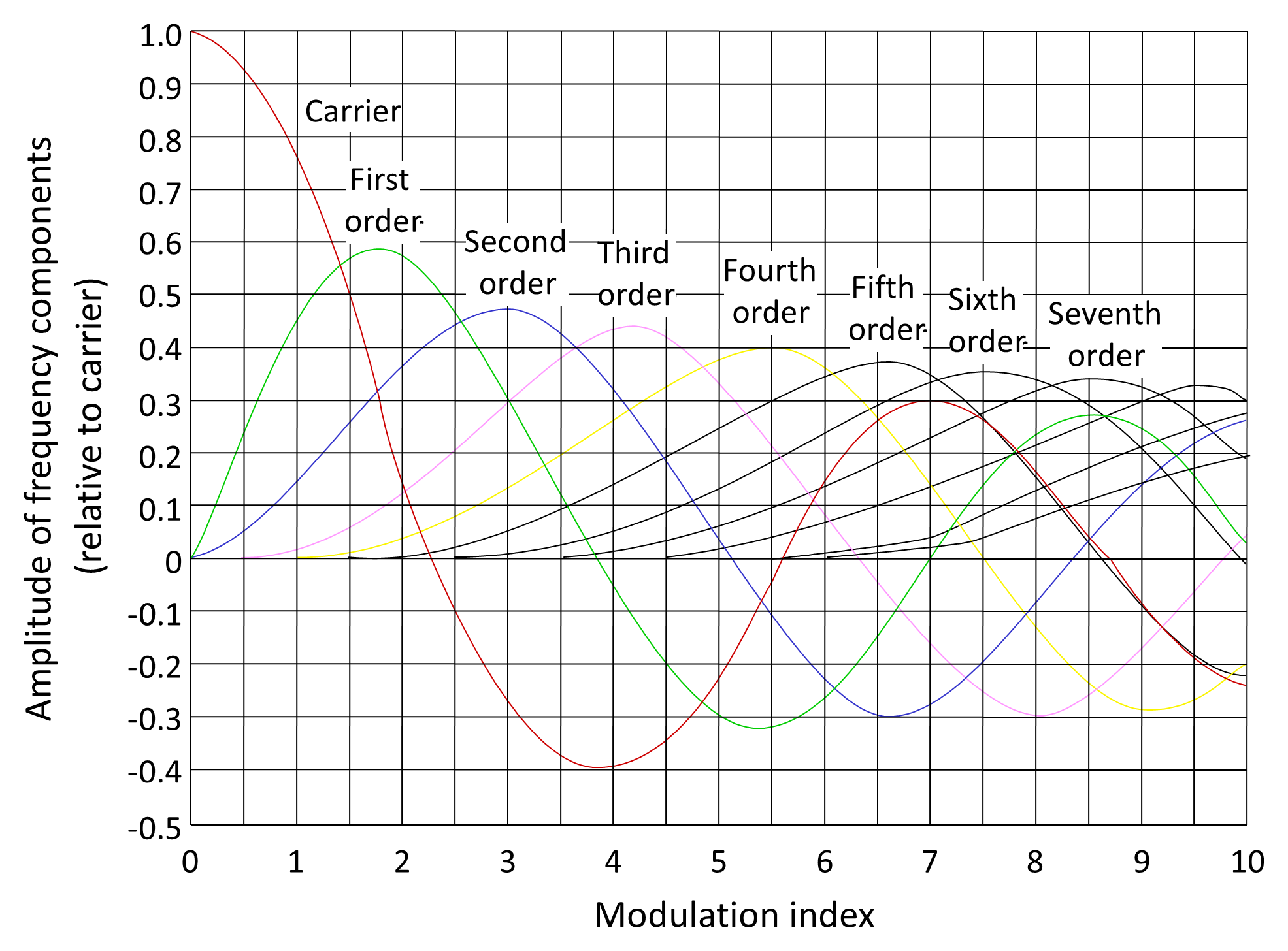
Figure 6.18. Amplitudes of the various frequency components of an FM wave vary with modulation index.

Some observations can be made regarding the form of Equation (6.33) and the frequency components illustrated in Figure 6.18.

Unlike AM, which produces only two sidebands for each modulating frequency, FM generates an infinite series of sidebands spaced f_m apart on both sides of the carrier frequency f_c. The first-order sidefrequencies are f_c ± f_m, the second-order side-frequencies are f_c ± 2f_m, and so on. Only the first few orders of sidefrequencies have been shown in Figure 6.18, but many more are possible.
The frequency components eventually decrease, but not in a straightforward way, fluctuating either side of zero. The change in sign of the magnitude indicates a 180° change in phase. Negative signs are normally omitted, however, since only the magnitude of each component is needed to consider its effect on the communication system.
Note that the carrier component varies in amplitude and is zero for some values of the modulation index. This is in contrast with full AM where the carrier is always present and remains constant.
The value of the modulation index is not constant but varies as the amplitude and frequency of the modulating signal varies. At any instant, the sidefrequencies will be f_m apart and the number of sidefrequencies, N, on each side of the spectrum is given by:

N \approx m_{f} + \sqrt{m_{f}} + 1

(6.34)

Values of N less than 1.5 are rounded down and values of 1.5 and greater are rounded up. Equation (6.34) illustrates that increasing the modulation increases the required bandwidth for faithful transmission. Figure 6.19 illustrates the frequency spectrum for an FM wave for m_f=2.