10.1 TRANSMISSION LINE THEORY

Consider the simple transmission line in Figure 10.1. Regard the transmitter as a simple alternating current (AC) generator whose output terminals alternately go positive and negative at a frequency of f Hz. As time progresses from the instant of switch-on, the “bunches” of electrical charge move down the transmission line in the direction indicated in Figure 10.2.

Figure 10.1. A simple transmission line.

Figure 10.2. Movement of charge down a transmission line with each half-cycle transition of the AC transmitter.

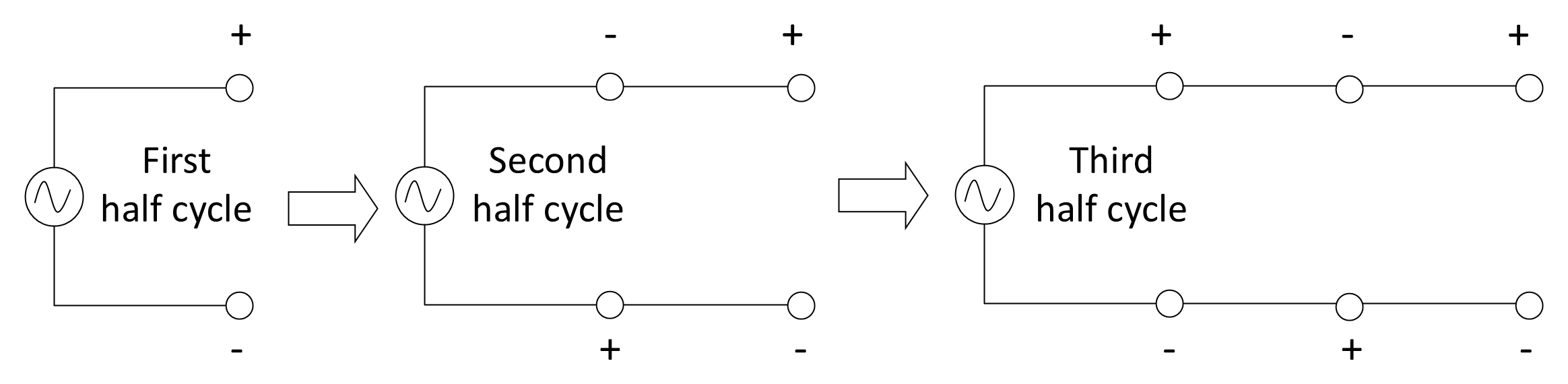
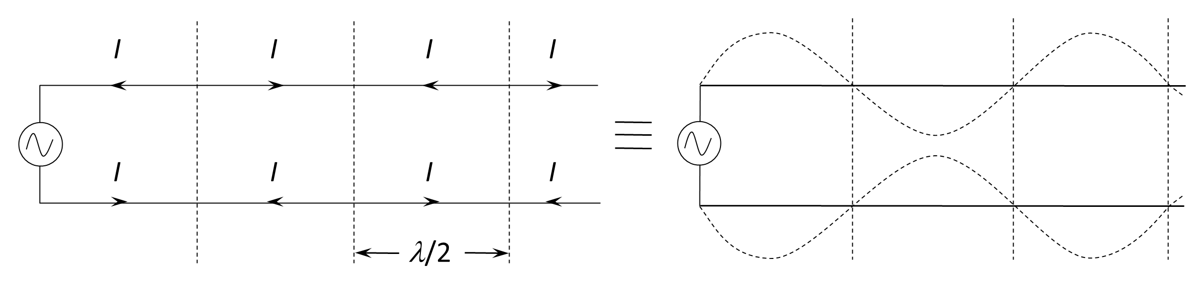
Since movement of charge constitutes current flow, this alternating motion is equivalent to a wave of alternating current propagating along the transmission line. If its peak value is I amperes, the instantaneous situation may be represented as shown in Figure 10.3.

The current propagates away from the generator with a velocity of propagation v_p m s^–1 and wavelength λ. The two are related by the fundamental relationship introduced in Chapter 2:

v_{p} = f λ

(10.1)

Figure 10.3. Current flowing down a transmission line.

Unlike free-space waves, which propagate without physical constraint, the wave on a transmission line is a guided electromagnetic wave, whose velocity depends on the effective permittivity of the surrounding dielectric medium.

The velocity of propagation of electromagnetic energy along a transmission line is generally less than the speed of light in free space because the electric and magnetic fields interact with the dielectric medium surrounding the conductors. The effective permittivity (and, in some cases, permeability) of this medium determines the propagation velocity. Different transmission-line types—such as open-wire line, coaxial cable, or optical fiber—therefore exhibit different propagation speeds depending on their dielectric composition and geometry. See Section 11.3 for a more complete explanation.

Typical propagation velocities for a range of common transmission-line media are shown in Figure 10.4.

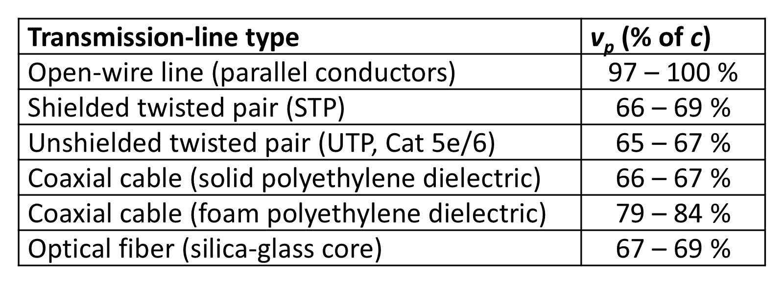
Figure 10.4. Approximate velocities of propagation of electromagnetic energy in various transmission media.

If the transmission-line environment changes—for example, from open-wire line to coaxial cable—the propagation velocity vₚ also changes, and if the frequency f remains constant, the wavelength λ will change accordingly.

There must also be a corresponding voltage wave travelling down the line. If its peak value is V volts, then:

\frac{V}{I} = Z

(10.2)

where Z is the characteristic impedance of the line. This impedance depends on several factors, including the spacing and diameters of the conductors, the properties of the dielectric, and the nature of the termination. Z may be purely resistive or may include reactive components due to the line’s inductance and capacitance. It should be noted that Z is not the same as the resistance that would be measured with a direct-current ohmmeter. It is important to distinguish between the characteristic impedance Z₀, which is a property of the line itself, and the load impedance Z_L connected at its termination. Proper operation requires that Z_L equals Z₀ to prevent reflections.

It is also useful to consider the fields produced by the current and voltage waves. In this context, a field refers to the region in which the electric and magnetic forces associated with the wave act upon a charged particle or a magnetic needle. These fields carry and transfer the energy of the wave along the line.