2.2.1 The Sinusoid

The sinusoidal function (also called a sinuate or sinusoid or sine wave) is the most convenient building block for signal analysis—it is simple to describe, and easy to handle mathematically and electronically.

Even if you are not familiar with how this waveform is generated, you will probably recall from trigonometry that the mathematical sine function is defined as follows. Draw a right-angled triangle as shown in Figure 2.1. The sine of the angle θ (the Greek letter theta—see Appendix A for a complete list of Greek letters and their English equivalents) between the hypotenuse and the adjacent side of the triangle is defined by the trigonometric ratio:

\sin (θ) = \frac{o p p o s i t e}{h y p o t e n u s e}

(2.1)

The two sibling ratios are also shown in Figure 2.1: cosine (cos) and tangent (tan).

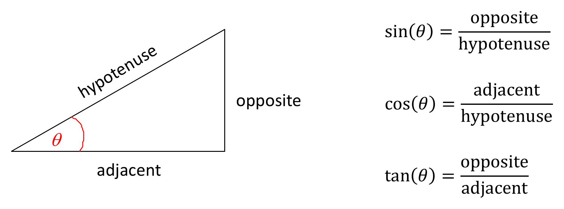
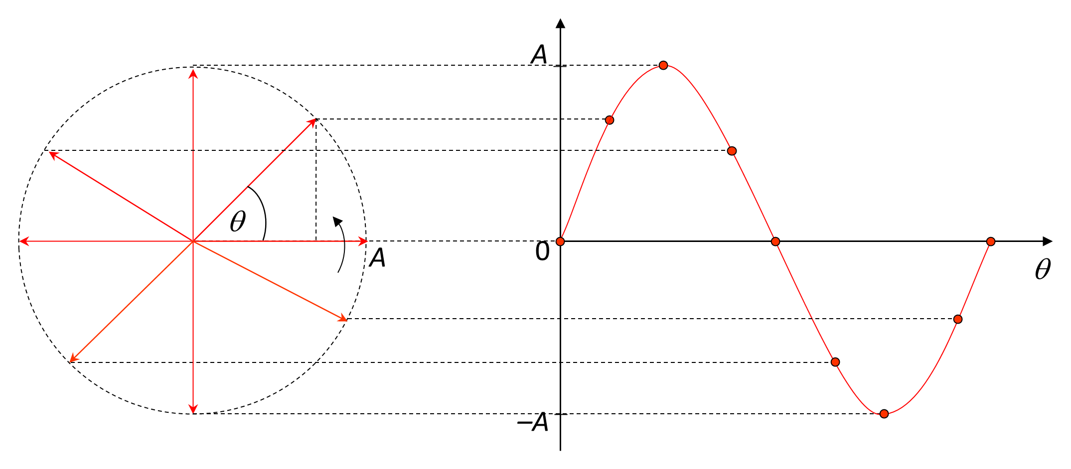
Figure 2.1. A right-angle triangle and the ratio relationships between sides and angle.

Consider the angle θ in Figure 2.1. If the length of the hypotenuse remains fixed, variations in the angle will result in variations in the height of the opposite side. Figure 2.2 shows the sinusoidal waveform that is the result of plotting the vertical height of the opposite side as a hypotenuse of length A is rotated around a circle by varying θ—the height is 0 when θ=0°, is A when θ=90°, is 0 when θ=180°, and so on. Note that the waveform in Figure 2.2 is the result of one rotation of the hypotenuse around the circle—that is, it is the result of one period of rotation.

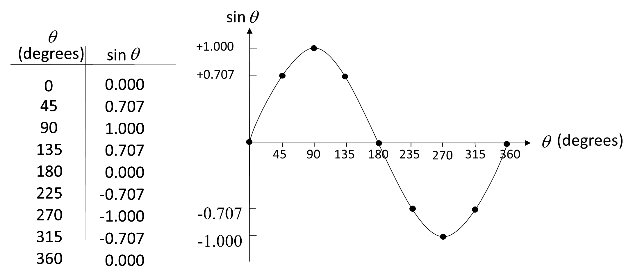
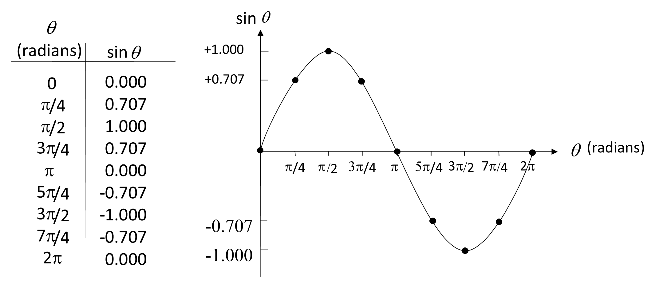
Figure 2.2. A sinusoidal waveform that is a result of plotting the vertical height of the opposite side of a right-angle triangle as the hypotenuse of length A is rotated by varying angles of θ.

When θ is measured in degrees, it ranges from 0° to 360°. Figure 2.3 shows how the sine function (sin θ) varies with θ (in degrees). The angle can also be expressed in radians (rad), where there are 2π radians in a circle (that is, in 360°). Figure 2.4 plots sinθ versus θ in rad. From the two figures, you can see the equivalence between degrees and radians: π/4 rad ≡ 45°, π/2 rad ≡ 90°, π rad ≡ 180°, 2π rad ≡ 360° and so on. We make the distinction because radians are much more useful to us during mathematical analysis.

Figure 2.3. Variation of the sine function (sin θ) with θ in degrees.

Figure 2.4. Variation of the sine function (sin θ) with θ in radians.

More generally, a sinusoidal waveform takes the form:

y = A \sin (θ)

(2.2)

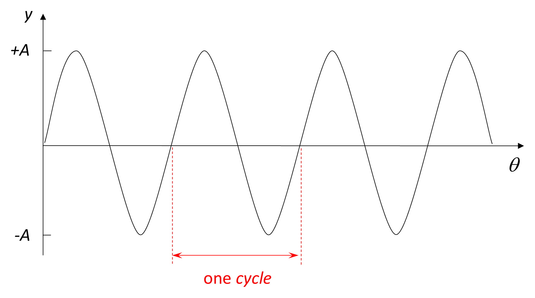
where A is the amplitude (or magnitude) of the sine wave as shown in Figure 2.5, varying symmetrically between magnitudes of +A and –A. The waveform is periodic, repeating every cycle. This periodicity is very useful to us. Not only is the sine wave simple to analyze mathematically but, because it is periodic, analysis can be confined to one period of the sine wave, while remaining valid for all time.

Figure 2.5. A simple sinusoid of the form y = A sin (θ).

A sinusoidal voltage, current, or electromagnetic wave can be described in two equivalent ways—either as a function of distance (how far the wave has travelled) or as a function of time (how the wave varies at a fixed point). These are known respectively as the distance model and the time model.

2.2.1.1 The Distance Model

One way to visualize a wave is to observe its variation with distance—as we might when viewing ocean waves from a clifftop. In this model a wave (let’s consider a voltage wave) can be expressed as a travelling sinusoidal function of distance:

v (x) = V_{m} \sin (x)

(2.3)

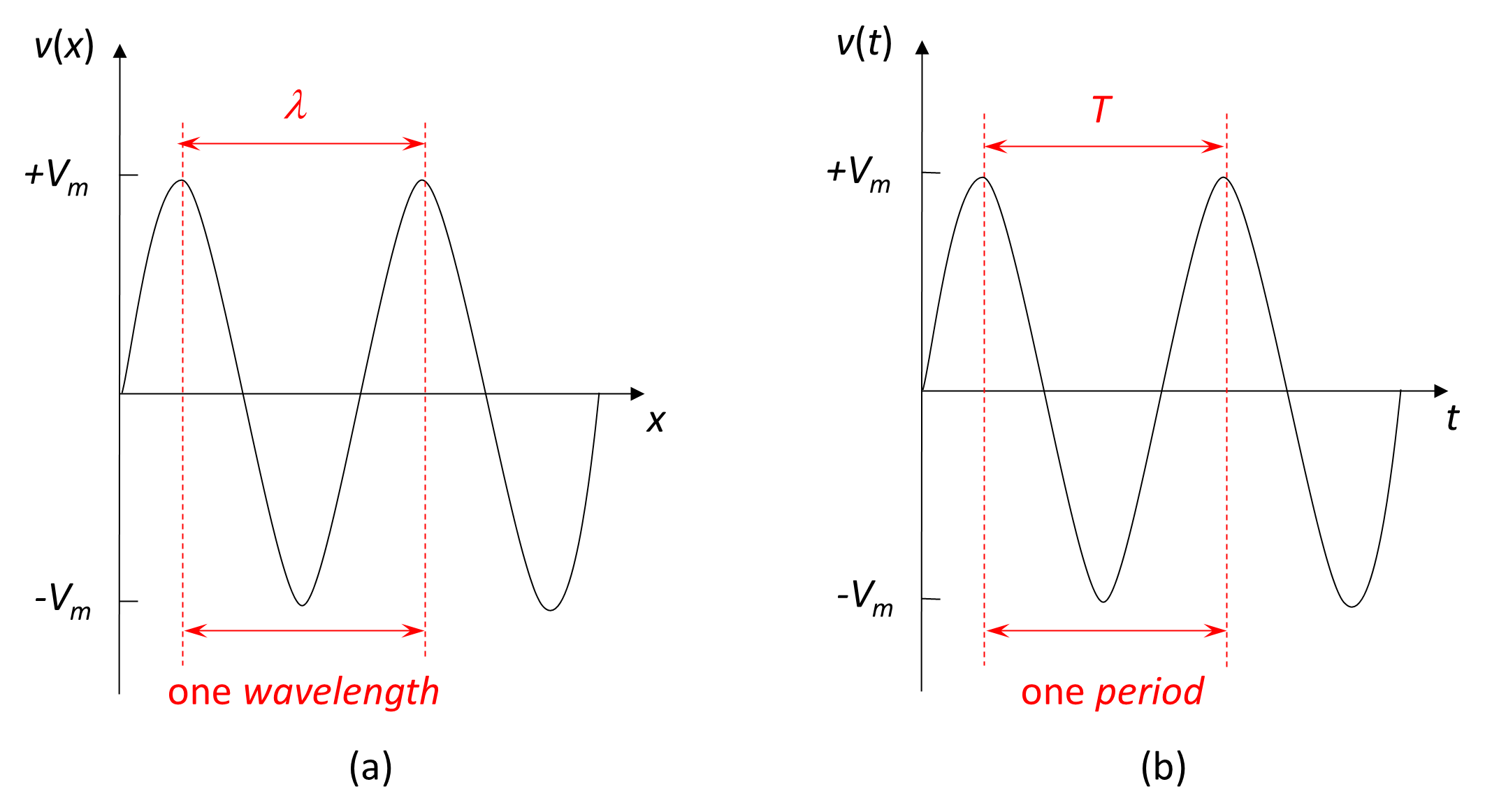
where v(x) is the signal voltage at a particular point in space, x (the script v denotes a varying quantity dependent on the variable x), V_m is the peak (maximum) amplitude of the signal voltage (the Arabic V denotes a quantity that does not vary—a constant, and the subscript m denotes the maximum value), and x is the distance travelled. Figure 2.6(a) demonstrates the relationship.

This model is useful as it highlights the physical properties of the wave, in particular its wavelength, λ (the Greek letter lambda—see Appendix A), which is measured in meters. As shown in Figure 2.6(a), and as the name ‘wavelength’ suggests, λ is the distance between successive points of equal amplitude (for example, from peak to peak) along the propagating waveform. Since the waveform is regular, its wavelength can be measured in a number of ways, but perhaps the most intuitive approach is to measure from peak to peak.

Figure 2.6. The electromagnetic wave a) as a function of the distance it has travelled, and b) its time varying nature.

2.2.1.2 The Time-Varying Model

While wavelength is a spatial property, in communications systems we often consider the wave’s variation with time, as this time dependence carries the information exchanged between the source and the sink. That is, given that we are at a particular point in space, we want to know what the wave looks like as it travels past us over time. Continuing the ocean analogy, this corresponds to an observer floating in a boat and recording their rise and fall over time at a fixed point. Figure 2.6(b) shows this time-varying sinusoid.

Two key quantities describe this time-varying behavior: period (T)—the time in seconds for one complete cycle; and frequency (f)—the number of cycles per second, measured in the units of per second (s^–¹) or hertz (Hz), named after Heinrich Hertz. Clearly, the two quantities (the time it takes to complete a cycle and the number of cycles per second) are inversely related:

f = \frac{1}{T}

(2.4)

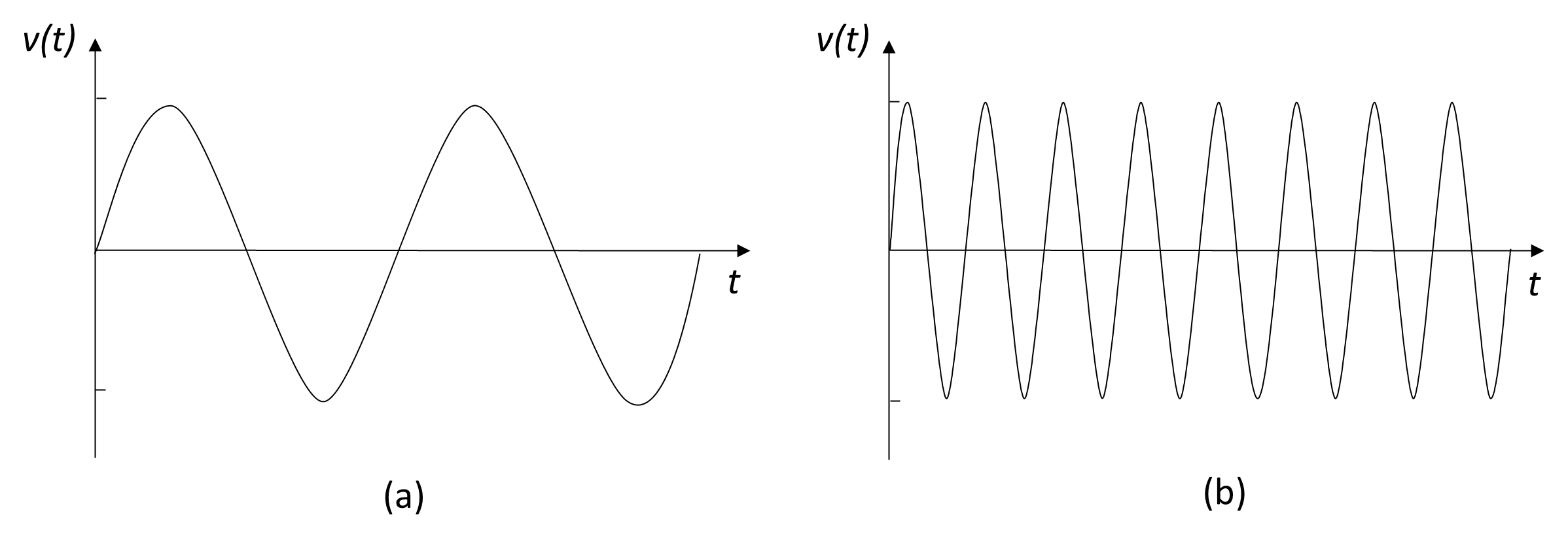
A high-frequency wave therefore completes more cycles per second than a low-frequency wave, as illustrated in Figure 2.7.

Figure 2.7. A sinusoidal wave of (a) low frequency, and (b) high frequency.

Example 2.1

A sinusoidal wave has a period of 1 ms. Calculate its frequency. Using Equation (2.4):

$f = \frac{1}{T} = \frac{1}{1 \times 10^{- 3}} = 1,000 Hz = 1 kHz$

Example 2.2

A sinusoidal wave has a frequency of 10 kHz. Calculate its period. Again, using Equation (2.4):

$f = \frac{1}{T} \Rightarrow T = \frac{1}{f} = \frac{1}{10 \times 1 0^{3}} = 1 \times 1 0^{- 4} s = 100 μ s$

We now need to discuss a slightly more complicated issue—that of angular frequency (ω). Figure 2.8 shows how a sinusoidal wave is generated by a hypotenuse (we can now name it correctly as a phasor) of magnitude V_m rotating anti-clockwise at an angular frequency of ω radians per second. As we saw earlier, the sinusoidal shape results from plotting the vertical projection of the phasor against time. Just as linear velocity is equal to distance divided by time, angular frequency is equal to angle divided by time. Consequently, the angle of the phasor relative to the x-axis at any time t is ωt. We can therefore write the equation for the time-varying sinusoid in terms of the angle at any time, ωt:

υ (t) = V_{m} 𝑠𝑖𝑛 (ω t)

(2.5)

where v(t) is the instantaneous signal voltage at time t, V_m is the amplitude of the signal voltage, ω is the angular frequency of the signal.

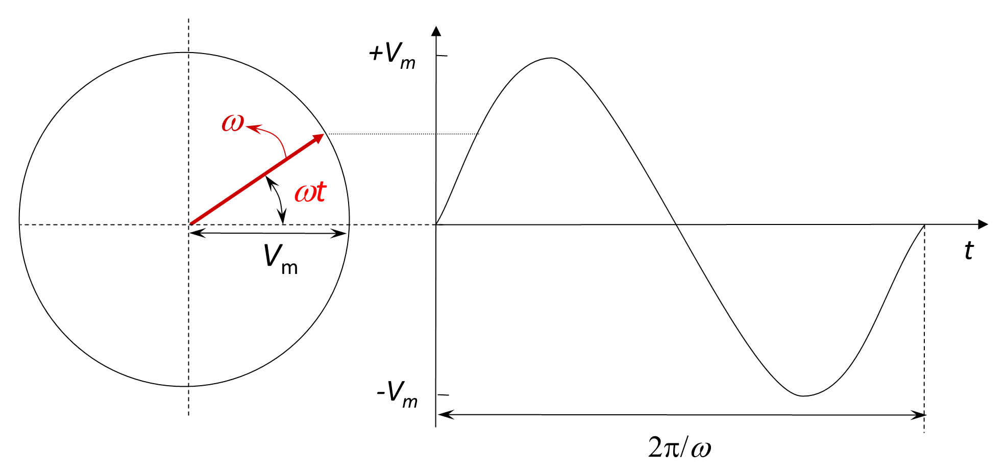
Figure 2.8. Generation of a sinusoidal wave by a rotating phasor of angular frequency ω and magnitude V_m.

One complete period (T) of the sinusoid is generated by one complete rotation of the phasor through 2π radians (or 360°). The time the phasor takes to complete the period is therefore 2π/ω, so the angular frequency (ω) is related to the period (T) by the relationship:

T = \frac{2 π}{ω} o r ω = \frac{2 π}{T}

(2.6)

Since T=1/f, we also have:

ω = 2 π f

(2.7)

Hence the time-varying relationship of Equation (2.4) can now be written as:

v (t) = V_{m} \sin (2 π f t)

(2.8)

In other words, if we know the frequency and maximum amplitude of a sinusoid, we can calculate the instantaneous signal voltage v(t) at any time t. We come back to this fundamental relationship a number of times in the following chapters.

2.2.1.3 The Relationship Between The Distance And Time Models

The distance and time models provide two complementary views of the same travelling wave, whether in free space or along a transmission line. Because both describe the same phenomenon, they are linked through one of the most fundamental relationships in wave propagation.

In the spatial view the wave repeats every wavelength, and in the temporal view it repeats every period T. Distance and time are related by the velocity of propagation v_p:

v_{p} = \frac{distance}{time} = \frac{λ}{T}

(2.9)

Since T=1/f:

v_{p} = f λ

(2.10)

For electromagnetic waves in free space, the propagation velocity equals the speed of light, c, which equals $3 \times 1 0^{8}$ m s^–1 (in Chapter 10, we note that the velocity of propagation along a transmission line is somewhat less than that in free space, typically ~75% of the velocity in free space). Thus, replacing for v_pin Equation (2.10):

c = f λ

(2.11)

or equivalently:

λ = \frac{c}{f} a n d f = \frac{c}{λ}

(2.12)

which are the two forms of the equation most commonly used.

Example 2.3

A sinusoidal wave travelling in free space has a wavelength of 10 m. Calculate its frequency. Using Equation (2.12):

$f = \frac{3 \times 1 0^{8}}{10} = 3 \times 1 0^{7} Hz = 30 MHz$

Example 2.4

A sinusoidal wave travelling in space has a frequency of 10 MHz. Calculate its wavelength. Again, using Equation (2.12):

$λ = \frac{3 \times 1 0^{8}}{10 \times 1 0^{6}} = 30 m$