4.6.1 Encoding
Convolutional encoders comprise a number of tapped shift register stages and exclusive-OR (XOR) gates (modulo-2 adders)—see Appendix E—that combine bits from selected register stages. Figure 4.18 illustrates the main functional blocks of an example convolutional coder with k=1 and K=3. Input bits are shifted progressively to the right through the register stages.
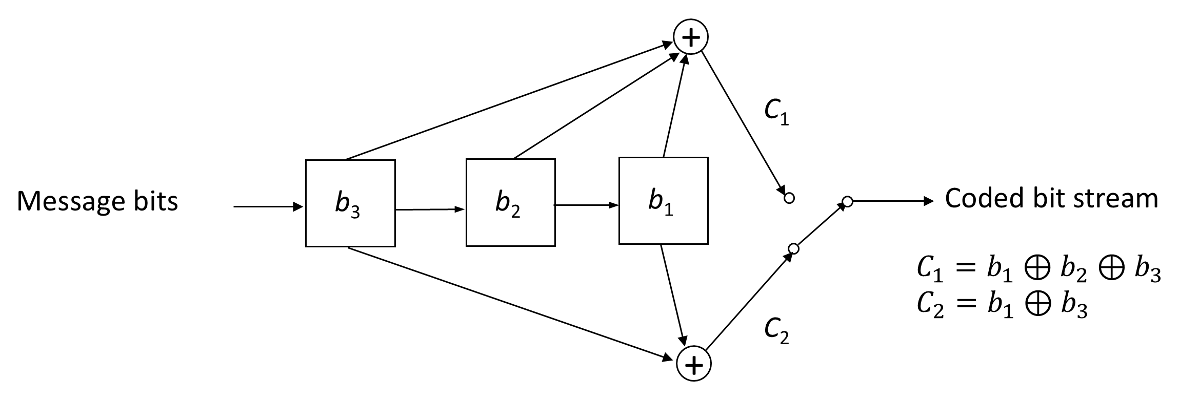
The outputs from the shift register stages are combined using XOR adders. Each information bit entering the encoder produces two coded bits, C1 and C2 given by
These bits are output sequentially and transmitted in order.
The coder is therefore a half-rate coder—for every input bit shifted into the register, two coded bits are created. The code generated by the encoder in Figure 4.18 is a non-systematic code; unlike block codes, non-systematic convolutional codes are preferred generally preferred because they yield better distance properties and simplify the design of soft-decision decoders.
Convolutional code rates are commonly 1/2, 1/3 or 3/4. Convolutional encoders are less efficient for very short messages because the shift register must be flushed at the end of the message by inserting (K-1) ‘0’s (known as the tail of the message). Consequently, the effective code rate is always slightly less than k/n.
The constraint length, K, of a convolutional encoder is determined by the number of stages on the shift register. In Figure 4.18, K=3. A half-rate coder with K=3 has a free distance of 5 and can therefore correct up to two bit errors.
Designing a convolutional encoder involves balancing error-correction capability (which improves with longer constraint lengths) against decoder complexity, which increases exponentially with K because the number of possible code branches grows as 2K. In practice, the optimal combination of shift registers and XOR taps is usually found by computer simulation or by consulting standard generator polynomials (e.g., NASA or CCSDS recommendations).
The coding process can be represented as a code tree, as illustrated in Figure 4.19 for a code with K=3 and rate 1/2. The encoder moves along a branch of the tree depending on whether the input is a ‘1’ or a ‘0’. For example, if the input sequence is “0101,” the encoder outputs “10 00 10 11.”
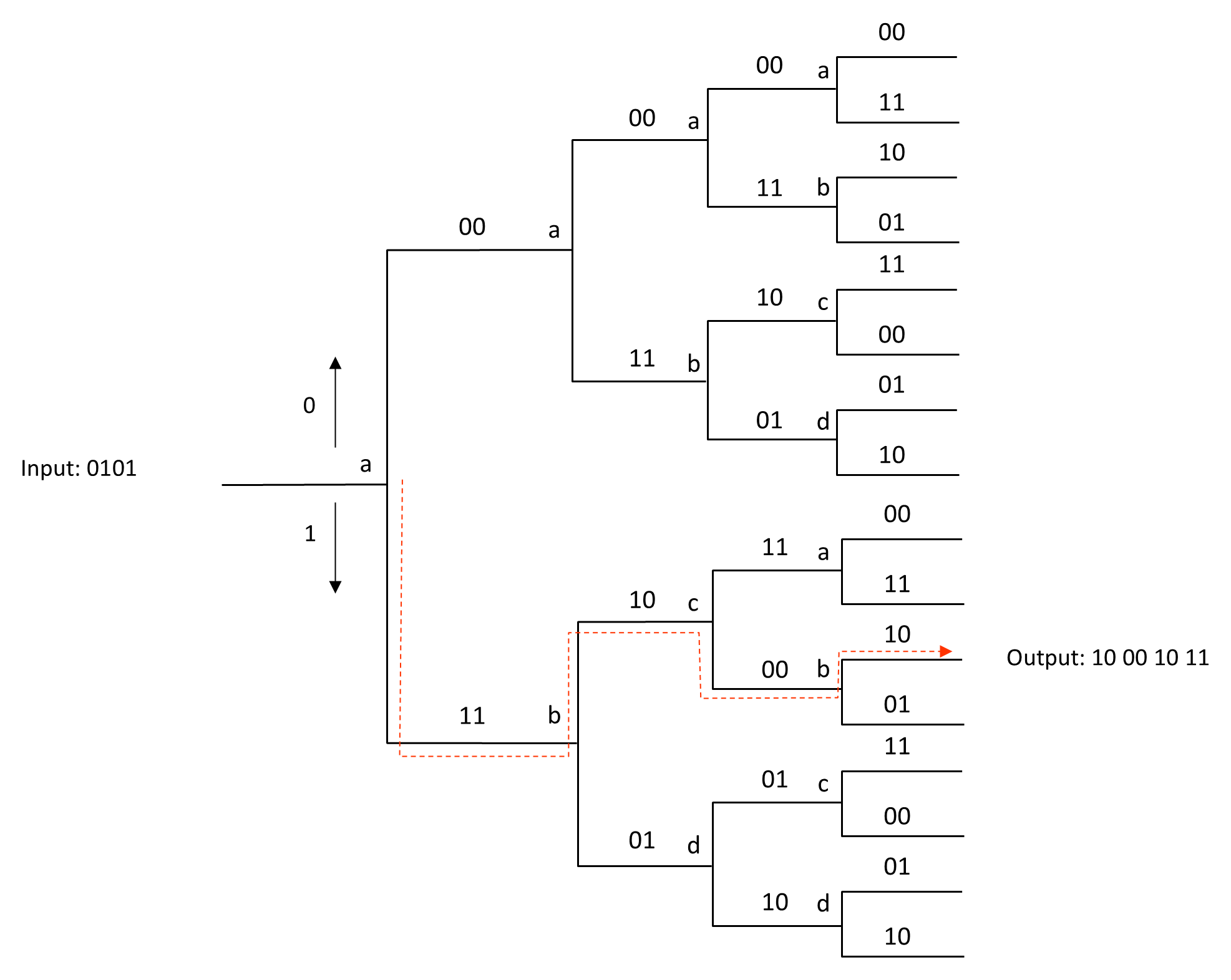
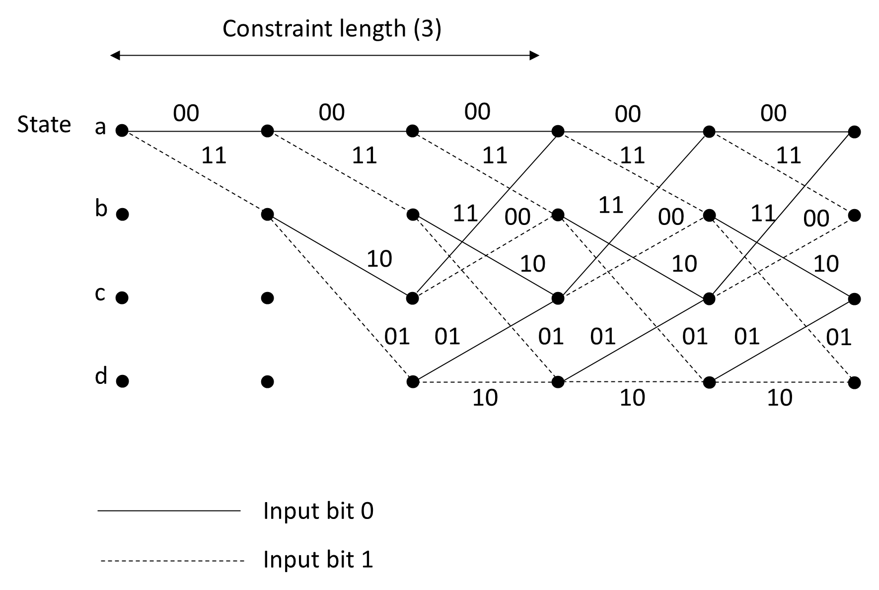
While the tree diagram provides an intuitive visualization of the encoder states, it becomes impractical for long input sequences. It can be observed in Figure 4.19 that the tree begins to repeat after K branches—the constraint length—since all branches leaving nodes of the same state (labeled a, b, c, or d) generate identical output sequences. These equivalent nodes can be merged to form the more compact and analytically useful trellis diagram.
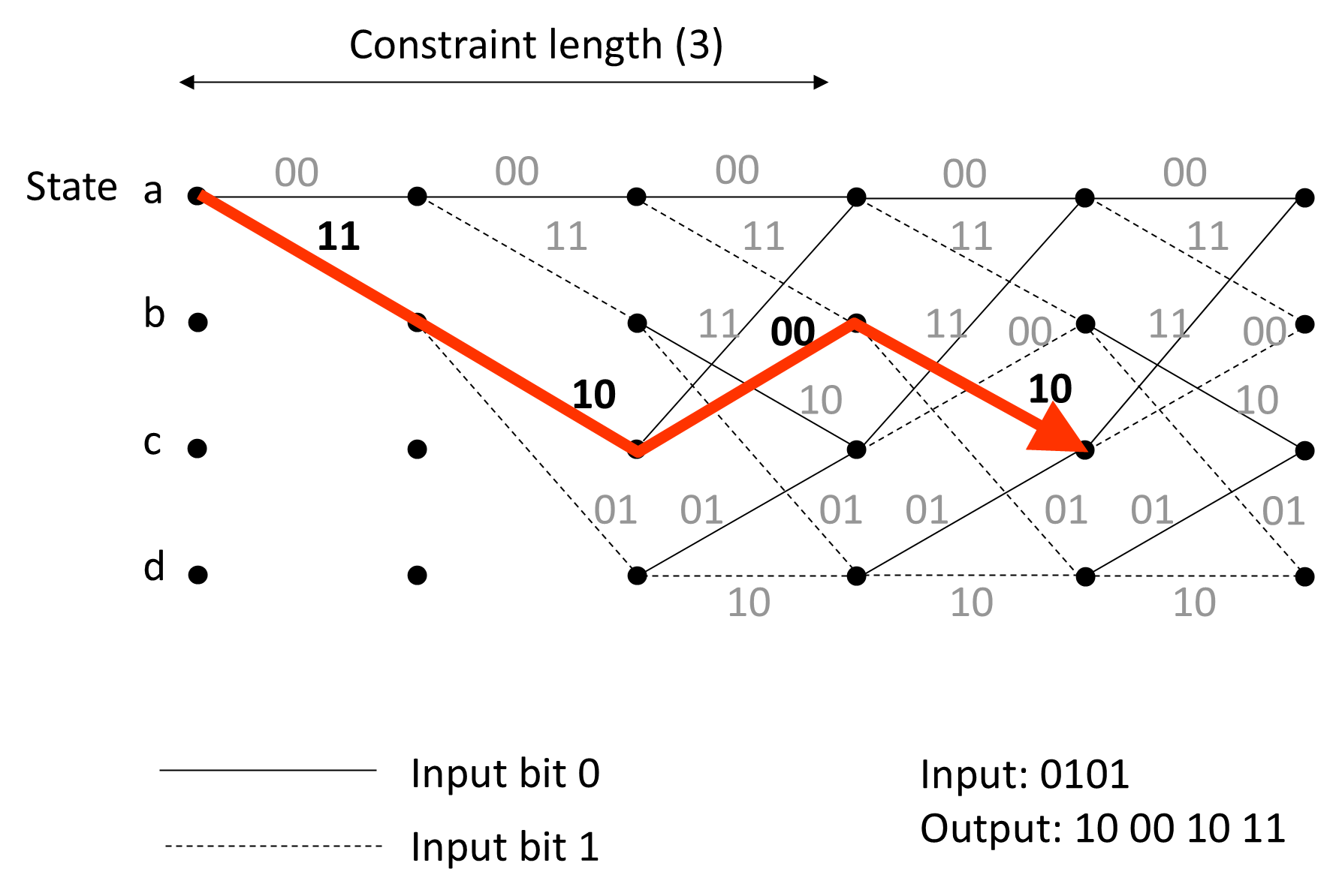
Figure 4.20 illustrates the basic building block of the trellis, corresponding to one state transition in the code tree. By convention, a solid line denotes the output generated by an input ‘0,’ and a dashed line denotes the output generated by an input ‘1.’
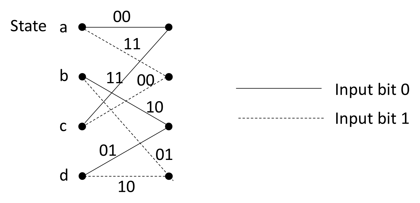
Figure 4.21 shows an expanded trellis with multiple state transitions, while Figure 4.22 the encoder’s output sequence for the input ‘0101’.
By exploiting the repetitive structure of the state transitions, the trellis diagram provides a compact and systematic representation of the encoder’s operation and serves as the foundation for decoding algorithms such as the Viterbi algorithm.