Military Aviation Applications For A Springs And Masses Safest Path Determining Model

Introduction

On the battlefield it is important to minimise the danger that personnel and equipment are exposed to. Achieving this involves routing around known or possible enemy threats. The route, or safe path, to be travelled is usually planned before a mission and is therefore based on what the threat environment looked like at some previous point in time. The complex and dynamic nature of the battlefield means that the threat environment that has to be travelled through, and therefore the safe path used, will almost certainly change. After the initial route is planned the decisions on how to traverse the threats that change en route have been made by commanders on the ground using their training and intuition [1]. This extra burden is less than ideal considering the other tactical decisions that compete for the commanders' attention. Incorporating a safe path determining computational model into battlefield systems alleviates this burden and allows commanders to focus their skills in other areas. Furthermore, there are an increasing number of Uninhabited Aerial Vehicles (UAVs) operating on the battlefield. These autonomous systems often have no commander available to make decisions about changes to the safe path. Without a computational model to perform this task, UAVs would be unable to adapt to changes in the threat environment without human assistance [2].

There are many situations where a safe path determining model can be employed on the battlefield. These include, but are not limited to, vehicles manoeuvring through a mine field, submarines avoiding both active and passive sensors so that they remain hidden and aircraft penetrating enemy air defence networks [3-5]. The last is the main focus of this work. The primary sensor in an air defence network is radar. Therefore, in order to penetrate enemy air defences it is essential for an aircraft to minimise its exposure to enemy radars, which minimises the danger the aircraft is exposed to. This makes the safest path synonymous with the stealthiest path and simplifies the problem of identifying threats because radars are active sensors.

The battlefield is a complex mix of different sensors with different capabilities, and this environment is in a constant state of flux; threats can change in relative danger, they can move or they can disappear or appear. Perhaps the greatest problem for safe path modelling is threats that appear near the current safe path, which are known as “pop-ups” [3]. Pop-ups can completely change the safe path. This means that a potentially dramatic change in the safe path must be re-calculated quickly in order to get around the pop-up with as little exposure as possible. It is this fast re-calculation requirement which causes the most difficulty for safe path determination computational models. The difficulty is compounded by the lack of computational power available on the battlefield. Military hardware must undergo rigorous testing processes before being introduced into service, so the computational power available is often much less than is available commercially due to the long delays in implementation [6]. Any safe path model that is to be used on the battlefield must therefore efficiently use the limited amount of computational power that is available.

There are many safe path determining models that can be used on the battlefield [7-14]. One of the most commonly used models is the Voronoi Diagram Search model. This model constructs a Voronoi diagram by drawing line segments which are equidistant to the nearest threats. All of these line segments are then searched for the safest combination which connect the desired start and end points. The model provides only an approximation for the safest path because of its discrete nature and because it assumes the safe path is half way between two threats. This is not necessarily the case if the threats have different relative dangers nor if there is a cluster of threats on one side and a single threat on the other. The model is of limited use in dynamic environments because every change in the threat environment is equivalent to starting the problem from the beginning, that is, re-calculating the entire problem, which is not an efficient method of adapting to changes particularly given the limited computational power available on the battlefield. Another common method is the potential field method [12-14]. Such an approach is commonly used in robotics where there are objective path/s and areas of avoidance (such as with other robot arms). However the key advantage of the springs and masses method (which we will describe in detail in the next section) is the length reducing component (the springs).

Springs and masses model

Most safe path determining models make a similar set of assumptions about the battlefield and threat environment. They begin by assuming that the threat locations are known. Threats are also considered to be isotropic, that is the danger level is the same in all directions around the threat. This is not an essential simplification as the Springs and Masses model can implement more complex threat types if desired. However, the assumption is maintained in this work because radars, the main threat that is considered, generally do act isotropically. Another main assumption is that the aircraft flies at a constant altitude and can only move in a horizontal two dimensional plane at that altitude. The altitude is arbitrary and is used only to set the vertical displacement of the aircraft relative to the threats so that range between the two can be accurately calculated. The model could also be adapted to three dimensions, but this is not done here for the sake of brevity.

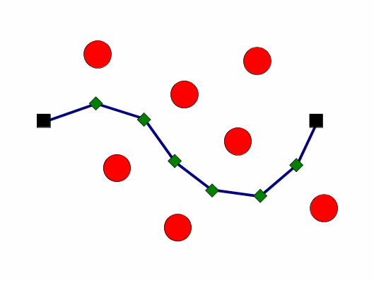
Previous work has found that the Springs and Masses model was best suited to the battlefield environment [1]. Figure 1 shows a simple example of the model. The model is constructed by placing masses between the desired start and end points. The masses are then connected into a chain using springs, and the two ends of the chain are anchored, one end at the start point and the other at the end point. The threats repel the masses with a force inversely proportional to a power of distance between them; the power is determined by the type of threat. The chain is now a large spring, mass and damper system, so the equations of motion for the i^th mass are described by the following equations:

${\dot{x}}_i{\text{=u}}_i$ (1)

${\dot{y}}_i{\text{=v}}_i$ (2)

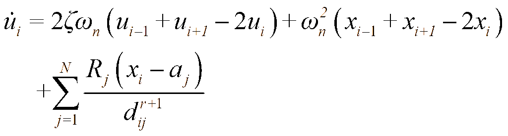
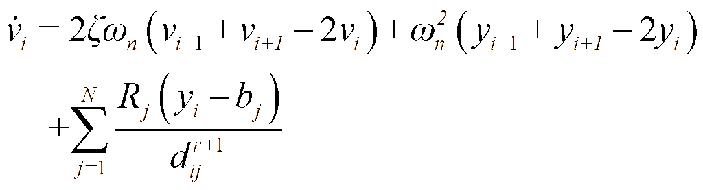
Equations (1) and (2) show the relationship between displacement and velocity. The location of the i^th mass is given by (x_i, y_i). The velocity in the x direction is u and in the y direction is v. Equations (3) and (4) are the standard equations for a spring, mass and damper system. The system has a damping ratio of ζ and a natural frequency of ω_n. The last terms in (3) and (4) are the forcing functions in the x and y directions respectively. The forcing functions are the forces acting on the masses from the threats. Assuming that there are N radars and the j^th radar is located at (a_j, b_j) with a danger level, or threat strength, of R_j. The distance between the j^th threat and the i^th mass is given by d_ij. The inverse power for the threat type is given by r. For radar threats the value of r=4 [1]. The line created by the chain of springs and masses when the motion of the masses has reached steady-state will be the safe path through the threat environment.

There are some short-comings with this basic model and these are discussed in detail by other authors (see [1,3,9]). Firstly, like many energy related problems, the chain of masses can reach steady-state at a local energy minimum. This will result in sub-optimum safe paths because the threat exposure is not globally minimised. Secondly, there is no in-built mechanism to restrict the length of the path, for example to account for vehicle range limits. There is also no measurement of the total threat exposure, which would be useful for risk analysis before beginning a mission. Fortunately, all of these short-comings have solutions, which have been implemented in the model used for this work.

The main benefit of using the Springs and Masses model over others is its efficient and computationally cheap method of adapting to changes in the threat environment. The appearance of a pop-up threat simply adds an extra force on all of the masses, but the force acting on masses far away from the new threat is small due to the inverse power of distance relationship. This means that most of the masses will still be in equilibrium and will not move, so no computational power is wasted on them. Masses close to the threat will only need to move a short distance until they again reach steady-state. This local updating of the areas of the path that need updating reduces the computational cost of updates. Further efficiency can be achieved by ignoring all of the forces acting on any masses that have already been passed when traversing the route. This means the model will not waste computational power updating the location of masses that are no longer important. The fixing of the travelled path is an improvement over other models which must continuously move the start location to achieve the same result, a process which involves re-solving the whole safe path. Finally, since the Springs and Masses model does not involve graph searching, there is no computational time wasted on combinations of path segments which are out of range of the vehicle. This problem was identified in many discrete models [11].

Another advantage of using the Springs and Masses model for battlefield applications is that it can offer very rapid part solutions for new safe paths as needed. This is because the model uses numerical integration to converge on a steady-state solution, which allows each integration step to be displayed as it is calculated. The converging nature of this time integration allows commanders to quickly see where the model might reach steady-state, and this may be all of the information that is needed to make a decision. Other models consider an exhaustive combination of path segments or initial conditions before returning the best. Using these models a commander must make an uninformed guess about what the model will eventually decide is the new safe path. The Springs and Masses model provides a better alternative, because even if the higher computational efficiency does not allow for a full solution to be calculated between display refresh times, the commander has an indication of where the new safe path will be.

Military aviation applications

One of the applications for safe path determining models is for aircraft penetrating enemy air defence networks. In such a situation, reducing the exposure of the aircraft to enemy sensors and the missiles that they guide will allow the aircraft to prosecute targets with relative impunity. The aircraft will also be able to maintain the element of surprise while achieving its mission objectives. Flying along a safe path requires continuous adjustments, which can distract the aircrew from their mission. Moving the burden of finding the safest path to and from a target to the mission computers will allow the limited crew of one or two people in an attack aircraft to either focus more on flying the aircraft or employing the aircraft systems, such as weapons. New generation fighters and UAVs are all attempting to simplify the numerous tasks that are needed to keep an aircraft flying safely, and using a safe path determining model is one possible simplification. The increasing adoption of Network Centric Warfare (NCW) based systems means that more information about enemy threats is available to more aircraft, but that information is worthless if it is not used to plan paths around the threats. All of these issues can be solved by implementing a safe path determining model, in particular the Springs and Masses model, in military aircraft.

Avoiding radars is a necessary condition for an aircraft to remain undetected because radar is the main method of detecting airborne aggressors. Therefore radars, rather than Surface to Air Missile (SAM) sites, are considered to be the threats for the safe path model. Fortunately, radars can be detected from further away than they are able to detect anything because of their electromagnetic emissions and reliance on returns (or echoes) from the aircraft they are looking for. The exact position of a radar can be found by sharing bearing information between other aircraft that have detected the same radar, or it can be estimated based on a single bearing and its signal strength. Other sensors, such as Infra Red Search and Track (IRST), should be avoided as well, but these sensors are passive and therefore harder to detect and route around. If intelligence or other means identify such sensors, they are easily incorporated into the Springs and Masses model.

The Radar Cross Section (RCS) of an aircraft may indicate that a minimum signal power must be reached before a radar can detect the aircraft, so there will be a corresponding minimum range that the aircraft must maintain from the radar site to remain hidden. The type of radar, or the radar's frequency band, can also indicate what type of weapon system it guides, and therefore the system's lethal range is known. These factors combine to give a relative danger level, or threat strength, that the model uses to modify the repelling force between the masses and threats such that the aircraft can remain as stealthy and safe as possible.

The battlefield for an aircraft is further complicated by objects that move, whether they are moving radars, targets or waypoints. Moving radars can be in the form of enemy fighters or enemy Airborne Early Warning and Control (AEWC) aircraft. Moving targets might be an enemy convoy or enemy bomber to be intercepted. Moving waypoints could be for aerial refuelling or landing on an aircraft carrier. The model used here simply moves these points with time and adjusts the safe path accordingly, although other more sophisticated implementation methods are also possible.

In order to stay updated with changes in moving points in this manner, the model must be computationally efficient enough to run at near real-time, otherwise the chain of masses will never reach steady-state. Currently an Euler time-stepping method is used to solve the system of ordinary differential equations (ODE). This technique was sufficient to solve the problem in near real-time because it only needs to calculate the repelling forces from the threats once for each mass at each time-step. Calculating the radar forces is the slowest part of the model because it must be repeated for each mass and each radar. Other models which use multiple steps for each part of the integration would need to calculate these forces multiple times, although the extra computational cost would likely be offset by taking larger integration steps.

Another factor which had a significant impact of the time to reach steady-state was the damping ratio of the springs and masses system. By setting the system to be over damped the kinetic energy of the masses is dissipated quicker, and therefore there are fewer oscillations as the chain of masses approaches steady-state. This results in the model finding a safe path quicker. Other gains in computational efficiency were achieved by ignoring the parts of the path that have been travelled and by displaying the path regularly, whether it was at steady-state or not. This last solution means that sometimes only a part solution is displayed, but as discussed earlier, this can be sufficient to make a decision to change the route. If the movement of the path with time is not sufficient to indicate that the model is displaying only a part solution, then indicator lights can be used that display some measurement of kinetic energy of the masses. When there is no kinetic energy the model has reached steady-state and the full solution is displayed.

Results

The code created for this work is designed to simulate the pathing problems for an aircraft departing from an aircraft carrier towards two targets and back to the aircraft carrier, which has moved to a new location. The code is capable of solving the initial problem before any points begin moving. It can then update the safe path as the aircraft progresses along the planned route. The code will also add random pop-ups to test the model's ability to adjust the safe path in real-time. The random nature of the pop-ups means that some will be very close to the safe path and others will be further away.

An example simulation is displayed in Figures 2 to 5. Figure 2 illustrates the initial safe path through the threat environment. The circles are the threats and their danger areas. The squares are the waypoints that must be reached, for example they may be targets that need to be engaged. The triangular shape represents the aircraft and it is currently situated on the aircraft carrier, which is denoted by the crossed lines. The line solid corresponds to the safe path that the model computes initially. The safe path clearly avoids all of the threats and reaches all of the objectives.

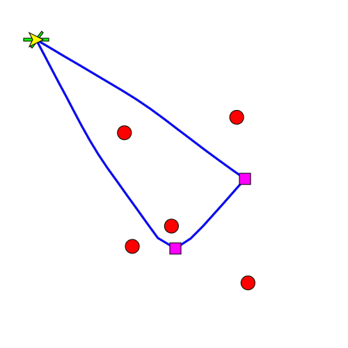
Figure 3 shows the situation after the aircraft has progressed along the safe path and detected a previously unknown threat close to the planned route between the objectives. The model has calculated the new safest path around the threat even before the aircraft has moved any further along the route, which is indicated by the aircraft still pointing in the direction of the previous safe path. This means the model found the new safe path within one refresh cycle, or less than one second. The aircraft carrier has moved away from the location where the aircraft departed and the safe path has been able to adapt to its changing position.

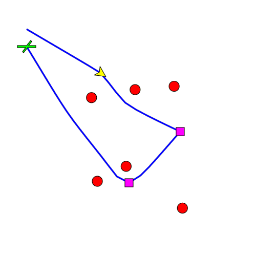
Figure 4 displays the situation after the first objective is reached. The aircraft has detected a new threat in front of it and near to the planned route to the second objective. The model has again updated the safe path within one second so that the new threat can be avoided. The path that the aircraft has already travelled along has not moved to account for the new threat because that part of the path is ignored for efficiency. The aircraft carrier has also moved further along and the path is still adapting to those changes in real-time.

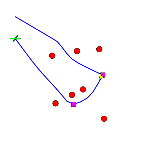
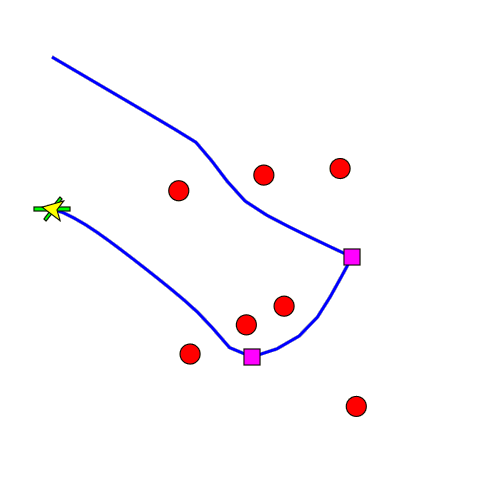
Figure 5 shows the end state of the mission. The aircraft has returned to the aircraft carrier and no more threats have appeared. The important feature to note is that the path between the second objective and the aircraft carrier is not a straight line even though there are few threats nearby. This occurs because the safe path is constantly moving while the aircraft flies along it. While the path that is travelled will be the instantaneous safest path between the two points, because the aircraft carrier is moving it will not be the overall safest path. A solution to this problem is to predict where the aircraft carrier will be when the aircraft arrives [15], and this is discussed in the following “Further Development” section.

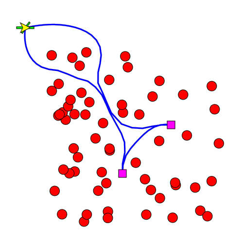
The model is not restricted to sparsely dispersed threats. Figures 6 shows an example mission with 60 threats. The safe path does not cross into the danger area for any of the threats and the path is within the range limits given to the model. Furthermore, the initial calculation time took only several seconds. Considering the complexity of the threat environment this is considerably fast and shows that the Springs and Masses model is flexible enough to be used in a wide range of situations.

Further development

The code used for this work was developed as a proof of concept only, not as an implementation. This means there are many more features and improvements that can be made. The efficiency of the code can be improved by implementing a more efficient solving technique. Previous work found that a combination of a modified Runge-Kutta ODE solver and a Broyden non-linear equation (NLE) solver was the fastest method of solving the large system of equations [1]. The code currently uses only an Euler time-stepping method, which is sufficient to achieve near real-time results, but is not the most efficient method.

Other improvements can be made in the physical modelling of the system. For example, including the third dimension into the safe path model to describe aircraft scenarios would result in safer paths because gaps in radar coverage at different altitudes could be exploited [11]. A similar benefit can be gained by implementing terrain masking effects on enemy radars. This would allow for paths that follow terrain features that block radar signals, potentially allowing aircraft to attack targets in heavily defended locations.

Other authors (see [5,9,11]) have implemented non-uniform Radar Cross-Sections (RCS) in their models to account for differences in radar returns depending on the orientation of the aircraft to the radar. Using non-uniform RCS is better suited to refining a safe path rather than finding an initial one. The feature is important because it makes a significant difference in the safe path through the threat environment. Implementing non-uniform RCS for the Springs and Masses model presents some challenges in finding the aircraft's orientation along the path because the masses are points and therefore have no orientation. This problem is solved in other models by averaging the orientation of the joining links, in this case the springs [9].

One problem with the current code is that, when moving waypoints have moved past a threat, the safe path remains on the original side, which adds both danger and length to the path.

If the moving point moves far enough that the springs are stretched to larger than the diameter of the threat, then the masses will slide across either sides of the threat. This allows the safe path to snap to the minimum threat area on the near side of the threat. For this technique to completely solve the problem, fewer masses must be used so that the average spring length is around the same as the threat diameter. However the safe path may then settle with the path crossing into a threat area. A better approach to the problem is to occasionally randomise the mass positions and solve the problem from the beginning once again. This would need to be preformed in the background so that the displayed safe path is not interfered with unless it needs to be changed. This allows the safe path to change which side of a threat is passed but still prevents the safe path from settling over a threat.

Another solution to the moving point problem is to predict where a moving point will be when the aircraft reaches it, and plan a path to that point. Using this method the model does not need to keep adjusting to the current location of the point and the path will not become stuck on the wrong side of a threat. The process would need to be iterative, because the Estimated Time of Arrival (ETA) depends on the path length. So when each path is found, the new ETA would need to be calculated, and then the location of the point at that time determined, then a new path to that point found. The computational efficiency of the Springs and Masses model allows these multiple iterations to occur relatively quickly. A similar approach has been used recently in a maritime surveillance setting [15].

Another use of predictive pathing is for coordinating Time Over Target (TOT) with other aircraft [2,16]. This allows for multiple aircraft to be tasked to achieve multiple objectives, and their speed and path are coordinated so that they all reach their objectives simultaneously. Such a strategy is useful for achieving complete surprise in an attack and does not allow the enemy time to react to prevent any of the attacks. This system has been shown to work using a modified Voronoi model [2]. The process for the Springs and Masses model would involve more iterations because there is a finer control over the path length than with the modified Voronoi model, which uses fixed length linkages.

A target allocation algorithm can be used to build on the coordinated TOT system. The target allocation algorithm could pool all of the targets and their relative priorities and then allocate targets to a pool of aircraft to attack. The safe path model would allow the algorithm to determine which target, or combination of targets, is safest or quickest to hit with which aircraft. An example of this type of system could involve ground units designating targets for an air strike then passing the coordinates to the target allocation system. The system would then find a UAV that is nearby that can safely reach the target and attack it, and then pass the target information to the UAV, which would use its own pathing system to find a route to the target. Potentially, the only humans in this process would be the people on the ground designating the targets. Such a system would allow ground forces to better employ air power and it would ensure that the available aircraft are used most efficiently. The feasibility of such a system has already been demonstrated [2].

At the moment the kinematic and dynamic constraints for the UAVs have not explicitly been taken into account. Such constraints may even make the paths no longer be realistic (flyable). We will consider this aspect in our future research into this problem.

Conclusion

Finding the safest path through a battlefield to achieve an objective is very important for military operations, particularly in the air. The main threats that an aircraft needs to avoid are the sensors that direct weapons to the aircraft's location, so the safest path is also the stealthiest path to the objective. In complex and dynamic environments a human may not be able to make good decisions about how best to avoid radars and other sensors, so offloading this task to a computational model not only reduces the burden on the people involved, but also provides better information. Previous work determined that the Springs and Masses model was best suited to these complex and dynamic environments [1]. However, while the model has proven to provide accurate information, it was previously unknown if the information could be provided in a timely fashion.

This work has focused on demonstrating a working Springs and Masses model that can solve safe path problems as near to real-time as possible. On a personal computer the model was able to find a complete solution between a single display refresh, which occurred at one second intervals. Modern military aircraft do not have hardware as fast as a typical personal computer, but the code is also far from optimised. With improvements such as using more efficient solvers and better programming techniques, the model could produce results in near real-time even on the minimal computational power available in military aircraft.

Another outcome of this work is that it has shown that the Springs and Masses model has tremendous potential for applications not only in military aircraft, but in many systems used on the battlefield. The model can be further developed to better simulate how threats affect aircraft, such as by implementing non-uniform RCS and terrain masking. It can also be extended to other applications such as ground and maritime operations. There is further potential for finding solutions faster by adding predictive aspects to the model to better account for moving points.

The Springs and Masses model has shown amazing depth and robustness in its simulation by modelling complex threat environments. Different types of threats with different features can be added to the model with relative ease and the effect they have on the safe path is shown intuitively as a force and displacement relationship.

As discussed earlier, there are still some improvements to be made to the system before a complete implementation of the Springs and Masses model is incorporated into a military aircraft, but the model has again proven to be suitable for the task. While the work that remains is largely implementation specific, there is still some generalised work needed in the areas of predictive pathing and threat modelling. All things considered, the Springs and Masses model is a powerful and flexible model that produces accurate and timely results. Even in its current state, the model should be strongly considered for implementation in combat systems in order to reduce the risk to both equipment and personnel.

References

Authors

Martin Rowe is an undergraduate in his final year of study for a BTech degree in Aeronautical Engineering. He is undertaking research projects as part of an enhancement program and upon completion of his degree he will be a commissioned officer in the Royal Australian Air Force.

Harvinder Sidhu is an Associate Professor of Applied and Industrial Mathematics at the School of Physical, Environmental and Mathematical Sciences, University of New South Wales at the Australian Defence Force Academy. E-mail: h.sidhu@adfa.edu.au

Geoffry Mercer is an Associate Professor of Applied and Industrial Mathematics at the School of Physical, Environmental and Mathematical Sciences, University of New South Wales at the Australian Defence Force Academy. E-mail: g.mercer@adfa.edu.au.

References

[1] M. Rowe, G. Mercer and H. Sidhu, “A Springs And Masses Model For Determining The Lowest Risk Path In A Threat Environment”, Proceedings of the 14th Biennial Computational Techniques and Applications Conference, submitted.
[2] R. Beard, T. McLain, M. Goodrich and E. Anderson, “Coordinated Target Assignment And Intercept For Unmanned Air Vehicles”, IEEE Transactions on Robotics and Automation, Vol. 18, pp. 911–922, 2002.
[3] G. Mercer and H. Sidhu, “Two Continuous Methods For Determining A Minimal Risk Path Through A Minefield”, Proceedings of the 13th Biennial Computational Techniques and Applications Conference, Vol. 48, pp. C293–C306, July 2007. Editors G.N. Mercer and A.J. Roberts.
[4] H. Sidhu, G. Mercer, M. Sexton, N. Ansari and Z. Jovanoski, “Optimal Path Trajectories In A Threat Environment”, Journal of Battlefield Technology, Vol. 9, No. 3, pp. 33-39, 2006.
[5] R. Murphy, S. Uryasev and M. Zabarankin, “Trajectory Optimisation In A Threat Environment”, Research Report 2003-9, University of Florida, pp. 1–48, July 2007.
[6] B. Ames, “Rugged Computers Power The Digital Battlefield”, Military and Aerospace Electronics, January, 2006.
[7] M. Jun and R. D'Andrea, “Path Planning For Unmanned Aerial Vehicles In Uncertain And Adversarial Environments”, Cooperative Control: Models, Applications and Algorithms (S. Butenko, R. Murphy, and P. Pardalos Ed), Kluwer Academic Publishers, pp. 95–111, 2002.
[8] M. Novy, Air Vehicle Optimal Trajectories for Minimization of Radar Exposure, Masters Thesis, Air Force Institute of Technology, Wright-Patterson Air Force Base, Ohio, 2001.
[9] S. Bortoff, “Path Planning for UAVs”, Proceedings of the American Control Conference, pp. 364–368, 2000.
[10] A. Dogan, “Probabilistic Approach in Path Planning for UAVs”, Proceedings of the 2004 IEEE International Symposium on Intelligent Control,, pp. 608–613, 2003.
[11] J. Leary, Search for a Stealthy Flight Path Through a Hostile Radar Defense Network, Masters Thesis, Naval Postgraduate School, Monterey, CA, 1995.
[12] L. Huang, “Velocity Planning for a Mobile Robot to Track a Moving Target – a Potential Field Approach”, Robotics and Autonomous Systems, Vol 57, No. 1, pp. 55-63, 2009.
[13] C.R. McInnes, “Velocity Field Path-Planning for Single and Multiple Unmanned Aerial Vehicles”, Aeronautical Journal, Vol 107, No. 1073, pp. 419-426, 2003.
[14] M.H. Mabrouk and C.R. McInnes, “Solving the Potential Field Local Minimum Problem Using Internal Agent States”, Robotics and Autonomous Systems, Vol 56, No. 12, pp. 1050-1060, 2008.
[15] G. Mercer, S. Barry, D. Marlow and P. Kilby, “Investigating The Effect Of Detection And Classification Range On A Simplified Maritime Surveillance Scenario”, ANZIAM Journal, Vol. 49, pp. C475–C492, 2008.
[16] T. McLain and R. Beard, “Trajectory Planning For Coordinated Rendezvous Of Unmanned Air Vehicles”, AIAA Guidance, Navigation and Control Conference, Paper no. AIAA–2000–4369, 2000.