
Volume 12, Number 1, March 2009
Intermittency Of Casualties In Asymmetric Warfare
- 1 Defence R&D Canada-Centre for Operational Research and Analysis, 101 Colonel By Dr., Ottawa, ON, K1A 0K2, Canada.
Abstract
Natural processes with long-term memory require a mathematical description with fractal (power-law) statistics. Two classes of such discrete processes that are of potential interest to the defence community are the fractal point process and the fractal rate point process. An analysis of fatality data from the conflicts in Afghanistan and Iraq is presented in this paper. The results reinforce the notion that there is a fundamental difference between the two conflicts, with the fatalities in Afghanistan behaving as a typical fractal point process with intermediate intermittency, while the fatalities in Iraq correspond to a fractal rate point process. These findings are supplemented by calculations of intermittency for several combat simulations. Implications of the results for the critical behaviour of the two systems, as well as future directions in terms of intermittency in models, are discussed.
Introduction
There have been a number of earlier studies demonstrating that the casualty numbers in regular and irregular warfare obey a power-law distribution (see for example [1,2,3]). Self-organized criticality was suggested as a possible mechanism behind this phenomenon. The presence of a power-law (fractal) size-frequency distribution in casualty numbers suggests the existence of a long-term memory in the system. This was further confirmed by the analysis of the long-term correlations in the fatality numbers from Afghanistan and Iraq [3].
There are a number of natural processes with long-term memory in physics, biology, and medical sciences [4]. Two classes of such discrete processes that are of potential interest to the defence community are the fractal point process (FPP) [5] and the fractal rate point process (FRPP) [6]. Use of the point processes as an analysis framework provides deeper insights into the dynamics of critical systems, and enriches the ability to assess risks connected with a particular mission. In particular, there is a connection between long-term correlations in a critical or sub-critical system and the likelihood of occurrence of an extreme event [7].
Since systems with long-term memory obey a power-law, rather than normal, distribution, the standard descriptive statistics (such as mean or standard deviation) do not have their usual meaning. The probability of extreme events is much higher than would be expected from a normal distribution. Therefore, the approach to assess the likelihood of events needs to be different. This paper presents one such possible approach of characterizing fractal systems. In particular, it addresses the intermittency as a measure of deviation from “expected” behaviour. For example, a conflict in which there is an occasional fatality, with long periods of no fatalities would be deemed intermittent, while a conflict in which there are large numbers of fatalities every day, distributed mostly uniformly, is not intermittent. In this fashion the knowledge of intermittency can contribute to estimation of a likelihood of fatalities.
This paper is organized as follows. At first a class of discrete processes called point processes is described. Then a means of describing intermittency and long-term correlations of point processes is summarized. Afterwards the methodology is applied to results of combat simulations, and to the coalition fatality numbers from Afghanistan and Iraq. Lastly, the implications of the findings are discussed.
Point processes and intermittency
In general, a point process is defined as a representation of a sequence of events N(t) on a time line. The methodology used below applies to stationary point processes, which are defined as point processes independent of the time origin t0. In terms of distributions N(t,t+Δt):

One important characteristic of point processes is the intermittency. A sequence of events is called intermittent if its dynamics sometimes deviates from the usual behaviour [4]. Sudden, positive deviations increase the mean of a sequence to values much higher than the most probable value. An example of such dynamics can include sudden spikes in a child’s activity as illustrated in [4], or, in terms of casualties, to sudden spikes in casualty numbers.
Bickel [4] proposes the use of the correlation co-dimension as a measure of intermittency. The method of characterizing intermittency is applicable to the analysis of near-critical systems, and as such it applies to casualty numbers. There is an alternative definition applicable to turbulent systems [8], but it does not apply directly here. The methodology is briefly summarized here; for detailed arguments on the use of the correlation co-dimension refer to [4].
The correlation co-dimension C2 is related to the second moment of the counting process:
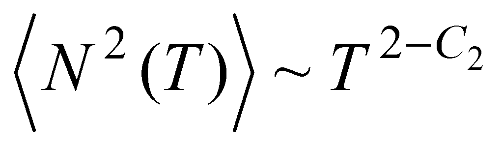
The correlation co-dimension values range between 0 and 1. The value of 0 corresponds to a non-intermittent process, while the value of 1 corresponds to maximum intermittency. Typical intermittent processes have values between the two extremes, which imply that they are fractal processes.
It is calculated as follows. It is assumed that there is an experimental time series {Z1, Z2, …, Zn} sampled at time steps T0. At first, a counting process is created:
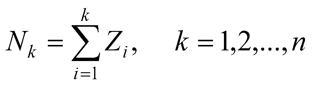
Afterwards, the variance <N2(T)> at times T=kT0 is estimated using a maximum-overlap estimator Sk for all k = 1,2, …,kmax ≤ n:

Finally, the value of 2–C2 is estimated from the regression of the slope of log Sk versus log T.
For FPP the co-variance relates to the Fano factor, defined as the ratio of the variance to the mean:
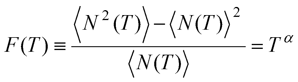
Comparison with (2) yields an equation connecting the co-dimension with the Fano factor:
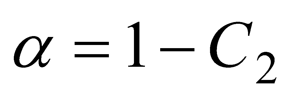
However, (6) does not hold for FRPP. In the case of FRPP, if there are long-term correlations present in the time series (such as for fractal Brownian motion, or for critical systems), the Fano factor is related to the Hurst coefficient H [4] as [1]:

The Fano factor can be estimated in a similar fashion as the correlation co-dimension. The counting process (3) for an experimental time series {Z1, Z2, …, Zn} is used to estimate the Fano factor using maximum overlapping windows as [1]:
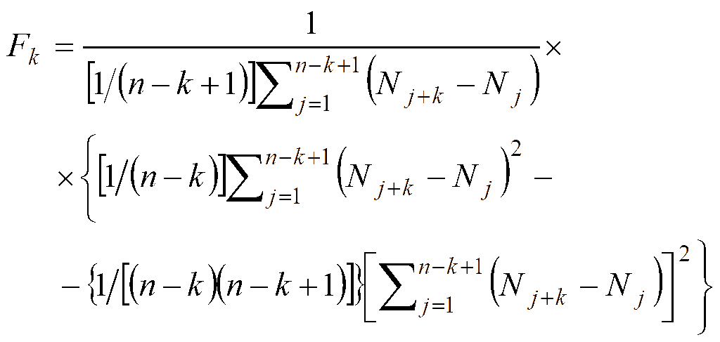
Then α is estimated from the regression of the slope of a plot of log Fk versus log T. It can be the used to either verify that the process under study is a FPP (that is, (6) holds), or in the other case (FRPP), provide an estimate of the Hurst coefficient H.
Intermittency in combat models
At first the intermittency of parameters obtained from combat modeling was analyzed. Notional scenarios were developed in MANA, an agent-based model (ABM) developed by New Zealand Defence Technology Agency (DTA) [9]. ABMs allow for generating large numbers of data by replicating the scenarios many times. This capability was utilized to generate data for subsequent analysis. Two different scenarios were modeled. Scenario 1 did not include any force manoeuvres, while Scenario 2 considered the BLUE force manoeuvring through an area occupied by an opposing RED force.
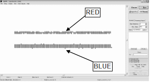
Scenario 1 featured an encounter between two large forces where all soldier entities were given the same individual firepower. The forces faced one another within ballistic and detection ranges. Combat consisted of a simple exchange of fire until one force was eliminated. Two options (Scenario 1A and Scenario 1B) were modeled: Scenario 1A considered equal force strengths while Scenario 1B considered unequal forces. In the former, two forces of 200 soldiers each were simulated. The single-shot kill probability (SSKP) was set to the same value for both forces (1%). In Scenario 1B, the BLUE force was twice the RED one (400 and 200 soldiers respectively), and the kill probabilities were lower (0.1%). The values for the kill probabilities were selected such that in 500 steps one of the forces would be almost completely eliminated, on average. Figure 1 shows the screen capture of the MANA scenario used to model Scenario 1B. All of the soldiers have unlimited ammunition supply, and they continue firing until killed. There is no force movement involved; the entire force disposition is static.
These configurations both satisfy the conditions of the Lanchester equations [10], and there was no reason a priori to expect any significant deviation from the analytical solution. Significant deviations from the Lanchester equations were observed and are mainly attributable to the discreteness of the MANA model. While the analytical equations assume that each of the forces is continuous and that each infinitesimal force element spreads its firepower over the entire enemy cloud, in reality each of the discrete agents engages only one opponent at the time, selecting the closest targets first.
The Lanchester equations (dB/dt = −kRR, dR/dt = −kBB) have an analytical solution that can be written in the form:


In (8) and (9), R0 and B0 denote the initial force strengths for the RED and BLUE force respectively, and:

For equal forces, (8) and (9) simplify to:


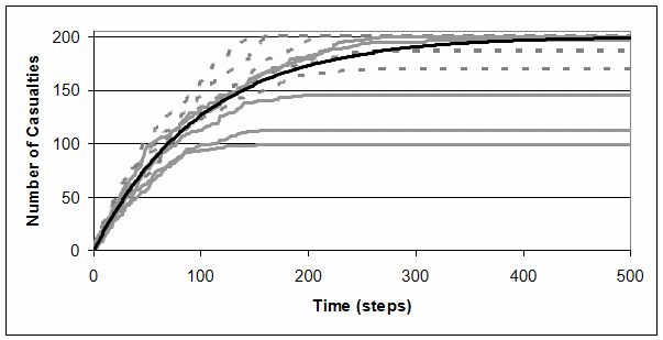
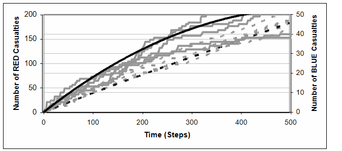
A comparison of theoretical and model results appears in Figures 2 (Scenario 1A) and 3 (Scenario 1B). The comparison was carried out using five independent MANA runs. For Scenario 1A (equal forces, Figure 2), there was an observable difference between the theoretical prediction and the modeling outcome. The reason was that the equations predict uniform attrition, while in reality early in the simulation one side usually gained a small advantage that grew quickly over time, and thus was able to eliminate the opponent faster, reducing its own casualties.
For Scenario 1B (unequal forces, Figure 3) the results mostly agree with the Lanchester prediction, the differences being largely due to the stochasticity of the model. An additional factor is the discreteness of the MANA model, as discussed previously. For instance, if BLUE created holes (regions of high attrition) in the RED line, the result would be a lack of RED return fire closest to these gaps. This could in turn lead to lower than expected BLUE casualties from the continuous forces mindset.
Below, the intermittency of Scenarios 1A and 1B is calculated via the co-dimension and the Fano factor for both BLUE and RED forces.
For Scenario 1A, the intermittency of the casualties for both forces was expected to be approximately equal. To calculate the co-dimension, a relationship between the length of a casualty sequence, and the cumulative number of casualties was obtained. The scaling obeyed a power-law relationship, leading to the values for C2. The intermittency for the BLUE casualties was about C2~0.22–0.27, and for the RED casualties it was in the range of C2~0.17–0.27. The Fano factor for the BLUE casualties was in the range of α~0.63–0.70, and for the RED casualties α~0.53–0.69. The results for the Fano factor are not consistent with the values that would be expected for the FPP. These values of the Fano factor suggest a correlated process, with the Hurst coefficient H~0.9. This is consistent with the observation that the outcome depends strongly on one of the sides gaining a slight advantage early in the simulation.
For unequal forces (twice as many BLUE as RED), the difference between the intermittency of RED and BLUE casualties was obvious. For the RED casualties the intermittency was C2=0.23, and for the BLUE casualties it was C2=0.35. This was consistent with the fact that the greater combat strength of BLUE led to increased and more uniform RED attrition. The Fano factor for some of the runs was impossible to determine (it was close to zero). For the runs where it was calculable, the values for both RED and BLUE casualties were approximately ~0.4. This is far from values that would be expected for an FPP. The low values for the Fano factor (and consequently the suggested values of the Hurst coefficient close to 0.5) suggest that, unlike the equal force case, the occurrence of casualties was mostly uncorrelated in time. This is consistent with the assumption of the Lanchester equations that casualties are distributed uniformly.
Next, a set of dynamic scenarios involving force movement were modeled. In the first of these, Scenario 2, 200 RED were distributed evenly over a battlefield (300×300 pixels), and two groups of 25 BLUE each moved along predefined paths across the battlefield in a zigzag pattern. The range of RED and BLUE weapons was set to 50 pixels, and the kill probability 1%. The Lanchester equations do not apply in this case, since the RED force is not concentrated in a single area, and the weapons are not able to reach all opposing soldiers. A scenario screen capture is shown in Figure 4.
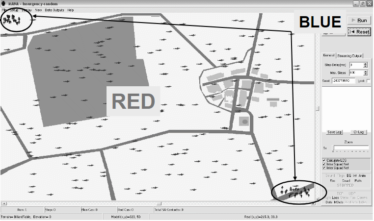
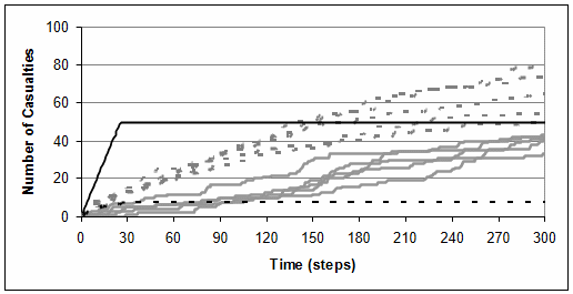
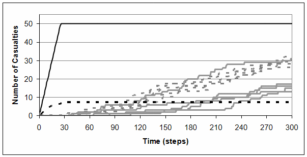
Scenario 2A assumed that BLUE would stay on their path no matter what, while Scenario 2B assumed that BLUE would actively pursue RED that they detected. The results for Scenario 2A are in Figure 5. Clearly the results differ to a great extent from the prediction obtained using the Lanchester equations. BLUE casualties were much more incremental, and RED casualties were much higher than predicted. The cause of the deviation was BLUE manoeuvring through the battle space and the fact that not all of RED were able to engage BLUE at the same time.
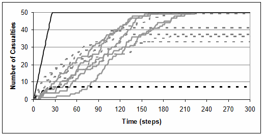
The results of Scenario 2B are in Figure 6. In this instance BLUE actively pursued RED, thus assuming a more distributed form as time progressed. In this way more targets were exposed to RED, and furthermore BLUE was not able to concentrate so much firepower either. This led to lower RED casualties, and a much faster increase in BLUE casualties compared to the first case.
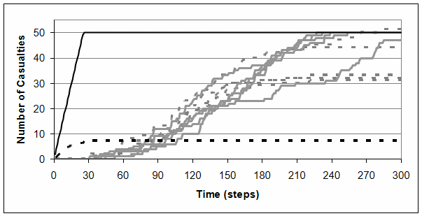
As an alternative, the same general scenario having a different RED disposition was modeled as well (Scenario 2C). In this case the RED force concentrated in small clusters. It was assumed that BLUE pursued RED when detected by them. This led to a slow initial increase in the number of casualties for both RED and BLUE, followed by a rapid increase in the casualty numbers. Next, the RED casualties are seen to plateau much earlier than the BLUE ones. This was caused by inadequate BLUE force strength. Overall, the result for BLUE was a sigmoid line.
A final variant (Scenario 2D) was modeled using a sparsely distributed RED force (50 soldiers divided into two separate, equal groups as opposed to 200 soldiers in all other scenarios). In this instance the number of casualties increased slowly, and the plateau was not due to an overwhelming strength of one side compared to the other, but rather it followed from the inability of the forces to eliminate each other. The RED casualties increased uniformly, while the BLUE casualties still followed a sigmoid curve. The difference was caused by the manoeuvring of the BLUE force that led to their ability to concentrate firepower and maintain uniform RED attrition.
As with Scenario 1, intermittency was estimated for all four options of Scenario 2.
In Scenarios 2A, B and C RED had a significant numerical advantage, therefore it was to be expected that the RED casualties would be more intermittent (less frequent and less uniform) than the BLUE casualties. If the BLUE force remained on their path (Scenario 2A), the encounters with RED were driven by the random distribution of the RED force on the battlefield. The occurrences of casualties were directly related to the encounters, and consequently they were rather intermittent. The co-dimension for the RED casualties was C2=0.45, and for the BLUE casualties it was around C2=0.31. As for Scenario 1, the relationship between the Fano factor and co-dimension valid for the FPPs was violated. The Fano factor for both RED and BLUE casualties was about α~0.3. This suggests that the casualties (and consequently the encounters) were actually slightly correlated.
For Scenario 2B (50 BLUE soldiers pursuing 200 RED randomly dispersed across the battlefield), the BLUE forces were eliminated faster, and thus their casualties were less intermittent, with C2=0.14. For the RED casualties C2=0.32. Again, the higher frequency of BLUE casualties was caused by RED’s numerical advantage. The Fano factor for both forces was higher than those found for the random encounters (α~0.4–0.5 for BLUE and α~0.3–0.4 for RED casualties). Thus the casualties appear slightly more correlated when BLUE pursues RED, compared to when BLUE simply follows their path (below).
For Scenario 2C (clustered 200-men-strong RED force in groups of around 15−20 soldiers, and the same BLUE force as above; BLUE pursuing RED) the results were not much different. This suggests that there is not much difference whether the RED are clustered or not; what matters is whether BLUE actively pursues RED or not. The intermittency of the BLUE casualties ranged between C2=0.14 and C2=0.17, and for the RED casualties between C2=0.32 and C2=0.38. This suggests that casualty intermittency was driven more by the kill probability than by the frequency of encounters. The Fano factor was almost the same for both forces, and it was in the same range as for the random RED distribution. This again suggests that the process is not a FPP, and that it is slightly correlated (H~0.7).
For Scenario 2D (clustered 50-men-strong RED force and BLUE in two groups of 25 individuals each), the intermittency of the BLUE casualties was significantly higher (C2=0.4–0.6), while the intermittency of the RED casualties decreased (C2=0.2–0.3). This was caused by the fact that in this instance RED were concentrated in smaller groups (about five soldiers), and thus BLUE were able to mass firepower and destroy more RED while minimizing their own casualties. The Fano factor for the RED casualties was α~0.5–0.6, and for the BLUE it was much lower α~0.2–0.3. This suggests that while the BLUE casualties were more random, the RED casualties were highly correlated with H~0.8. This corresponds to the difference in the shape of the casualty lines in Figure 8, as discussed above.
In summary, it appears that as long as the combat strength of the two sides during encounters is comparable, the intermittency is driven primarily by the kill probability, with little influence stemming from the actual force distribution and manoeuvres. This was confirmed by the observations of both the Lanchester case (Scenario 1) and three options for the dynamical case (Scenarios 2A–2C). However, if one of the forces can manage to mass firepower during the encounters (Scenario 2D), the intermittency is influenced by it, leading to lower intermittency of the stronger side and much lower intermittency (more uniform attrition) of the weaker side.
There have been a number of previous studies investigating deviations of MANA simulations from the Lanchester case [11,12,13]. The findings of these studies are consistent with the results presented above, namely, that the ability of one side to mass firepower can cause a significant deviation from the Lanchester prediction, and turn the balance of force in favour of an otherwise weaker enemy (insurgents, for example). This has a potentially significant implication for counter insurgency (COIN), especially if the COIN forces are distributed over large distances, and the insurgents have the ability to cluster their firepower in a particular area. This can lead to a localized, temporary increase of insurgent combat strength to the point that they could overcome the otherwise superior COIN forces.
Intermittency of casualties in afghanistan and Iraq
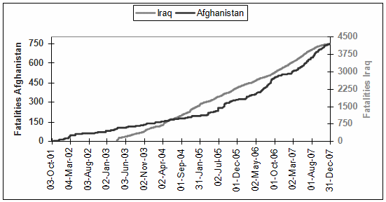
Actual conflict fatality data for the coalition operations in Afghanistan and Iraq are now analyzed. Only the coalition fatalities were included, since reliable and consistent information concerning insurgent fatalities in the encounters was not available. The fatality numbers for Afghanistan are sparser than those from Iraq. However, while the increase in cumulative coalition fatalities in Iraq is linear, the increase in the cumulative coalition fatalities in Afghanistan is exponential, and thus it is possible that the conflict in Afghanistan can become more deadly for the coalition than the conflict in Iraq (Figure 9). Dobias [3] showed that there is a difference in the nature of the two conflicts, in that the fatalities in Iraq exhibit characteristics of a critical system, while the fatalities in Afghanistan exhibit properties of a sub-critical system. Therefore it is reasonable to expect that the different nature would be reflected in different intermittency characteristics for the two conflicts.
To begin with, the coalition casualty numbers in Afghanistan are analyzed. The scaling factor obtained from the log Sk vs. log k dependence was 2–C2 = 1.64. This in turn implies a co-dimension of C2=0.36. In other words, the Afghan conflict yields medium intermittency of casualties. On the other hand, for the casualties in Iraq the scaling factor 2–C2 =1.90, yielding rather low intermittency (C2=0.10). In both cases the dependence was linear across the entire range of k, and the goodness of fit was estimated to be R2=1.00.
Next, the Fano factor was estimated for both conflicts. For Afghanistan, it was found that the dependence of log Fk vs. log k deviated slightly from linearity for both extremes of the range for k. The linear (middle) portion of the data series was used in calculating the Fano factor. The theoretical value (α=1–C2) was α=0.64. The value obtained from the Fk(k) dependence was α=0.61, close to the theoretical value, as is to be expected for an FPP. The goodness of fit for the selected interval was R2=0.99.
For Iraq, the dependence of log Fk versus log k is linear for most of the range with the exception of few points at either extreme. The computed value of α=0.38 is far from the value that would be expected for an FPP (0.90). This, combined with the low intermittency, suggests that the conflict in Iraq exhibits the properties of FRPP.
As mentioned previously, the Fano factor can be used to estimate the Hurst coefficient. Thus in the case of Iraq the value is H=(1+α)/2=0.69. This is in a qualitative agreement with the earlier findings [3] that analyzed the correlation in the coalition casualty data in Iraq and came to the conclusion that indeed the data exhibited long-term correlations (although the value that was obtained in [3], using detrended fluctuation analysis, was somewhat higher (up to 0.8)).
To summarize, there is clearly a qualitative difference in the intermittency of coalition casualty numbers in Afghanistan and Iraq. Casualties in Afghanistan are intermittent, exhibiting properties of an FPP, while casualties in Iraq exhibit very low intermittency, and correspond to the characteristics of an FRPP. The summary of the results is in Table 1.
Fractal nature of irregular warfare – relationship between modeling and observations
In an earlier study [3], the analysis of frequency/size scaling and of the long-term correlations suggested that both conflicts (Afghanistan and Iraq) are self-organized systems with Iraq exhibiting all of the characteristics of the critical state. On the other hand, coalition casualties in Afghanistan were anti-correlated, characteristic of discharge event systems [7]. The intermittency properties identified in this paper are consistent with the observations of the preceding study. The Afghan conflict exhibits rather intermittent casualties, which corresponds well to the anti-correlated system (an occurrence of a significant event in terms of casualties is bound to be rare). The power law scaling of the size/frequency relationship reinforces the findings that there is a relationship between the Fano factor and the co-dimension typical for FPP. For the casualty numbers in Iraq, the long-term correlations are well reflected in the low intermittency of the series. This is well corroborated by the value of the Hurst coefficient obtained from the Fano factor.
In summary, both analyzed representatives of irregular warfare (IW) exhibit characteristics of fractal processes. This includes power-law scaling of the variance with the interval size, reinforcing the suggestion that the IW can be described as a self-organized critical or sub-critical system.
Comparison of the factual attrition data with the attrition results of the constructive simulations (see the Section Intermittency in Combat Models, above) highlights another interesting aspect of the two conflicts. Inferring from simulation, since the intermittency of the Iraq conflict is quite low, it suggests that casualties are likely driven by the kill probability, and thus the firepower/survivability ratios for both the coalition and the insurgency are comparable. In further inference, the low intermittency of the coalition fatalities in Afghanistan, on the other hand, seems to be consistent with the situation whereby the coalition force can mass firepower against an opponent that does not have enough immediate combat strength to retaliate. In other words, the relationship between the insurgent firepower and the coalition force protection is more favourable to the coalition. This brings up an important consideration—an increase in the insurgent capabilities to defeat the coalition force protection might lead to a further rapid increase in the number of coalition casualties, yielding the system unstable, and prone to “explosive” instability (with the growth rate increasing with time) [14].
| Conflict | Co-dimension | Fano Factor | Hurst Coefficient | Fractal Process |
|---|---|---|---|---|
| Afghanistan | 0.36 | 0.61 | N/A | FPP |
| Iraq | 0.10 | 0.38 | 0.69 | FRPP |
Conclusions
The intermittency of fatalities was used to characterize tactical combat. The intermittency was calculated for several combat scenarios that were simulated using the agent-based model MANA. This allowed for control of the circumstances of combat, including the distribution of forces and also force manoeuvres so as to better understand the relationship between the intermittency and the dynamics of combat.
Subsequently, the intermittency of coalition fatalities for the conflicts in Afghanistan and Iraq were calculated and a qualitative comparison between the two conflicts revealed that the former is best characterized as an FPP and the latter an FRPP. Furthermore, comparison with simulation results suggested that casualties in Iraq are likely driven by comparable combat strength (in the terms of individual tactical encounters, not the overall theatre-level capabilities) for coalition and insurgent forces, whereas in Afghanistan the comparison of the combat strength in tactical encounters is more favourable to the coalition.
In previous work [3], it was demonstrated that the two conflicts are qualitatively different. These early findings were further confirmed and reinforced by the analysis of the intermittency.
Overall, the analysis points to a coalition force vulnerability. Specifically, should the insurgents increase their ability to focus firepower enough to match or even overcome the coalition combat strength, there could be a significant shift towards rapidly increasing numbers of coalition fatalities, especially in Afghanistan.
References
[1] D.C. Roberts and D.L. Turcotte, “Fractality and Self-Organised Criticality of Wars”, Fractals, 6, 1998, pp. 351−357.
[2] L.F. Richardson, “Frequency of Occurrence of Wars and Other Fatal Quarrels”, Nature, 148, 1941, pp. 598.
[3] P. Dobias, “Self-Organized Criticality in Asymmetric Warfare”, Fractals, Vol. 17, No. 1, 2009, 1−7, in press.
[4] D.R. Bickel, “Estimating the Intermittency of Point Processes with Applications to Human Activity and Viral DNA”, Physica A, Vol. 265, 1999, pp. 634−648.
[5] S.B. Lowen and M.C. Teich, “Estimation and Simulation of Fractal Stochastic Point Processes”, Fractals, Vol. 3, No. 1, 1995, pp. 183−210.
[6] S. Thurner, S.B. Lowen, M.C. Feurstein, C. Heneghan, H.C. Feichtinger, and M.C. Teich, “Analysis, Synthesis, and Estimation of Fractal-Rate Stochastic Point Processes”, Fractals, Vol. 5, No. 4, 1997, pp. 565−595.
[7] R. Woodard, D.E. Newman, R. Sanchez, and B.A. Carreras, “Persistent dynamic correlations in self-organized critical systems away from their critical point”, Physica A, Vol. 373, 2006, pp. 215−230.
[8] M.V. Stepanova, E.E. Antonova, A.J. Foppiano and T.J. Rosenberg, “Intermittency in the auroral absorption fluctuations as manifestation of magnetospheric turbulence”, Advances in Space Research, doi: 10.1016/jasr2005.04.112, 2005
[9] M.K. Lauren and R.T. Stephen, “Map-aware Non-uniform Auto-mata (MANA): a New Zealand Approach to Scenario Modelling”, Journal of Battlefield Technology, Vol. 5, No. 1, 2002, pp 27−31.
[10] F.W. Lanchester, “Aircraft in Warfare: The Dawn of the Fourth Arm. No. V, the Principle of Concentration”, Engineering, Vol. 98, 1914, pp. 422−423
[11] M.K. Lauren, “Firepower Concentration in Cellular Automata Models—An Alternative to Lanchester Approach”, DOTSE Report 172, NR 1350, 2000.
[12] G.C. McIntosh, M.K. Lauren, “Incorporating Fractal Concepts into Equations of Attrition for Military Conflicts”, Journal of Operational Research Society, 2007,
[13] M.K. Lauren, G.C. McIntosh, N. Perry, and J. Moffat, “Art of War Hidden in Kolmogorov’s Equations”, Chaos, Vol. 17, No. 1, 2007, pp. 013121−013126
[14] P. Dobias, J. Samson, “Nonlinear instabilities in magnetized plasmas: a geometrical treatment”, Canadian Journal of Physics, Vol. 82, 2004, pp. 593–608.
http://www.palgravejournals.com/doifinder/10.1057/palgrave.jors.2602383