Volume 10, Number 3, November 2007

Prediction Of Fragment Distribution And Trajectories Of Exploding Shells

Joanna Szmelter¹ and Chung Kiat Lee²

¹ Loughborough University, Leicestershire LE11 3TU, United Kingdom.
² Defence Science and Technology Agency, 1 Depot Road #18-05, Defence Technology Tower A, Singapore 109679.

Abstract

A semi-empirical model allowing for prediction of natural fragmentation of exploding shells is described. The initial velocity, projection angle, size and location, obtained for each fragment, are used by a point mass trajectory routine to determine the overall fragment distribution on the ground and to model fragments hitting a three-dimensional object. Examples of validation against experimental data for 105-mm shell and a mortar bomb are shown. The proposed model is useful for munition assessments, including a prediction of safety hazard in a credible accident.

Introduction

This study focuses on the natural fragmentation of shells. Although sophisticated numerical methods using hydrocodes are currently available for fragmentation prediction, these can be time-consuming to learn and require lengthy computation. Moreover, the reliability of prediction is sensitive to input parameters which are not readily (if at all) available. Here we describe a fast turn-around semi-empirical model.

Most of the available semi-empirical models have two major problems. Either they use Mott distribution in which case they fail to predict the actual fragment distribution or using an input distribution they fail to predict fragment velocity distribution. The proposed model employs different approaches. Two major elements which distinguish it are: the geometrical transformation featuring some nonlinear effects and allowing for initial velocity modelling in geometrically complex shells with varying case thickness; and the introduction of the empirically based classification of fragments to the natural fragmentation modelling methodology. The later alleviates any need for undesired model calibration.

In comparison with controlled fragmentation, designs relying on natural fragmentation provide the benefits of the low manufacturing cost and high strength during firing. However, for natural fragmentation mass distribution is difficult to assess. For a prediction of fragment mass distribution, the best known is the Mott equation [1]. References [2,3] provide a review of this and other methods based on statistical distributions. Such methods are largely concerned with finding a general distribution formula and omit specific information about physics related to a particular design. Consequently the models which use statistical distributions frequently require a calibration against experimental data, which reduces their predictive value. In contrast, the proposed method relies strongly on the varying magnitude and angle of the initial velocity of fragments as well as build of the shell.

Description of the model

Figure 1 shows a representative shell for which the proposed fragmentation model was developed. As in any reliable model it is important to provide an accurate geometry representation and for realistic shells, a CAD geometry should be used.

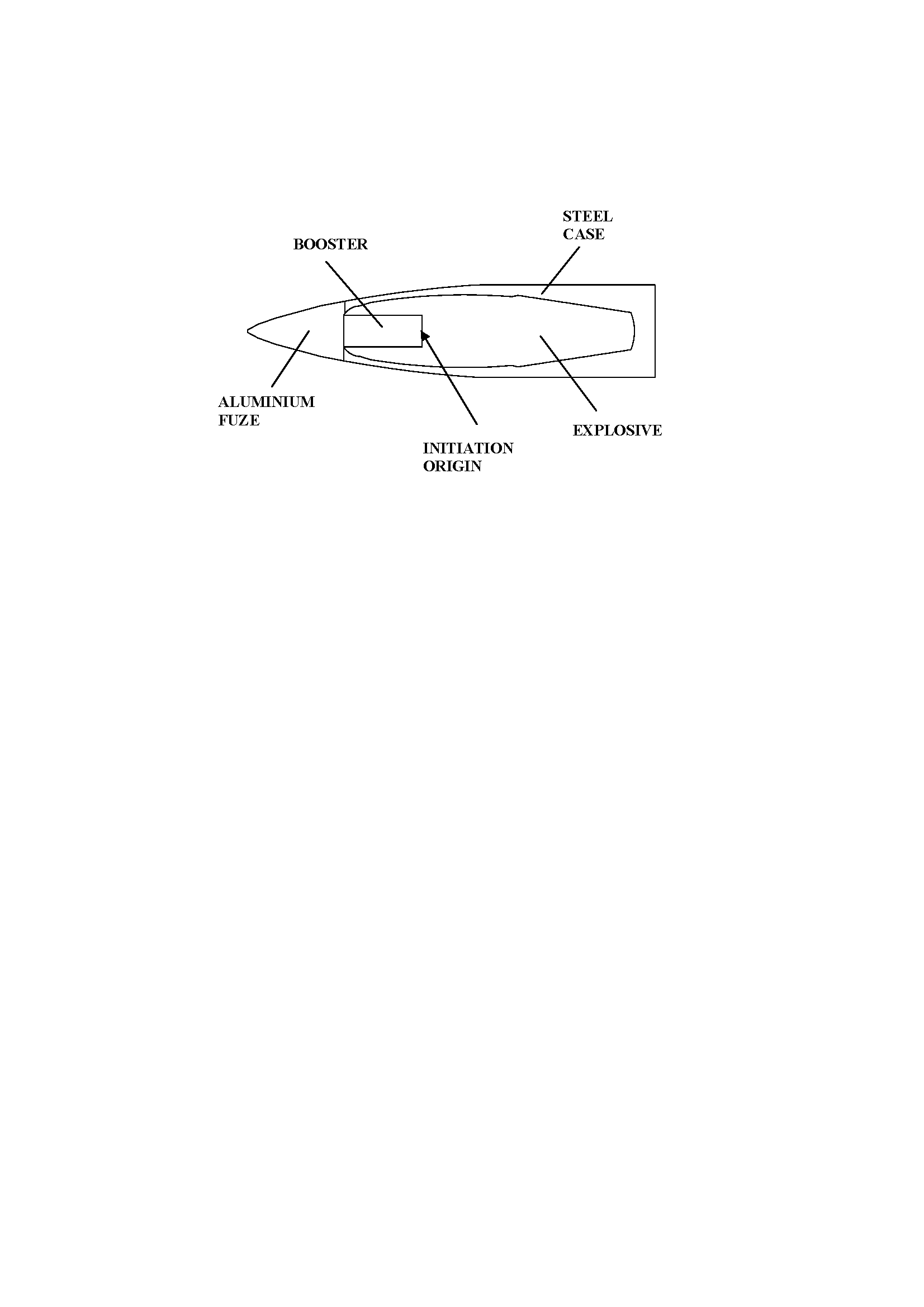
The wall (that is, fuze and case) of the shell is first divided into a number of computational elements. Our sensitivity study has shown that for a typical problem, illustrated in Figure 1, a division to 300 elements is adequate to eliminate the influence of numerical discretisation. Taking into account a safety factor, for a possible increase in the geometrical complexity, we ordinarily use approximately 500 elements. For every element the initial velocity and projection angle are calculated.

Since the first equations for prediction of fragment velocity for a sphere and an infinitely long cylinder based on the empirical data were formulated by Gurney[4], a range of equations valid for other simplified shapes have been proposed, for example, in various references [5,6]. For more complex shapes the formulation of an analytical equation becomes increasingly difficult. Occasionally, methods approximating a real shape by an infinite cylinder are used for estimation, notwithstanding introduction of approximation errors and ignoring kinetic energy loses in fuze and base regions. Some other reported techniques divide a shell into a set of short cylindrical segments and use the Gurney equation for every segment in turn. Such approaches need to be used with care as they are limited by the recognition that the Gurney equation is only valid for long cylinders.

For the calculation of fragment velocity of each element, we used an approach that very closely follows Jayaratnam[7]. The calculation of initial velocity is based on the transformation of the shell geometry into a hollow sphere, assuming constant charge mass and wall mass as well as constant surface area of the charge. Then the Gurney energy balance technique is applied [4]. The presence of the booster is taken into account during calculation of the filling mass. The method was further modified to account for a possible change in density for each segment of the casing [8]. A detailed description of the procedure employed in this paper is described in reference [8]. Compared to other standard semi-empirical modelling, the approach allows for more realistic simulation of a complex geometry of conventional shells with steel body and aluminium fuze. It appears to be fast and well-suited for shells of general shape and with walls of varying thickness.

The fragment projection angle is calculated based on the Taylor angle equation [9], linking detonation velocity, angle of the casing wall relative to the shell axis and fragment initial velocity.

δ_{α} = \frac{V_{α} cos (β_{α} - θ_{α})}{2 V_{D}}

(1)

where V_D is the velocity of detonation.

In order to improve the accuracy of the projection angle calculation, the correction [10] was implemented. The projection angle in the standard Taylor equation (1) depends on the expanding case velocity. In the generalised Taylor equation [10] corrective terms are added that also take into account the acceleration of the expanding case. The comparison of calculations using existing shells [11], revealed that in the context of our model this correction has negligible effects.

As a result the initial velocity and projection angle for every computational element (shown in Figure 2) is known. If velocities and projection angles of the neighbouring elements differ less then 5%, the elements are agglomerated to form a separate axisymmetric section of the wall (Figure 3).

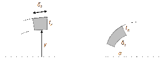
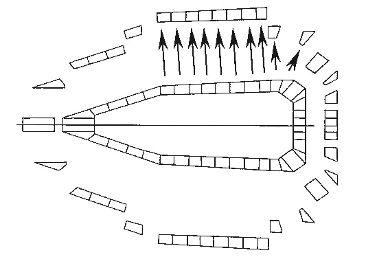
Figure 2. An element on the shell for which the initial velocity is computed.

Figure 3. Illustration of agglomeration of elements based on similar fragment velocities and projection angles.

Such a procedure is consistent with the physics of the problem, since the wall will tend to cleave first at locations where there is a considerable difference in fragment velocity or projection. The wall expands and develops cracks before breaking into fragments. When the agglomeration is complete, the shell is represented by a set of sections. Next, the fragmentation of every section is modelled separately, starting with a calculation of two typical distances between cracks on the internal surface of the wall. To account for the double curvature of the wall, the first distance is computed in the direction of the axis of symmetry and the second distance in the direction perpendicular to the first.

The two distances are estimated from the same equation proposed by Grady [12] and used as follows:

a_{i} = {(\frac{24 {Gr}_{i^{2}}}{ρ_{M} V_{o^{2}}})}^{\frac{1}{3}}

(2)

where: a_iis the average distance between cracks corresponding to curvature i (axial or circumferential) ; G is the energy per unit area to form a crack; r_i is the shell wall radius corresponding to the direction of a; ρ_M is the density of wall material and V_o is the initial fragment velocity. The resulting distances: a_x- a distance between cracks in the axial direction and a_yin the circumferential direction are indicated in Figure 4.

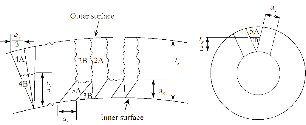
Figure 4. Illustration of type and size of fragment for the fracture mechanism corresponding to 2 < ratio < 3. Figure 4.Illustration of type and size of fragment for the fracture mechanism corresponding to 2 < ratio < 3.

Multiplication of a_x and a_yallows for the approximation of the area of the rectangular ‘breakage’ on the internal surface of the section. The number of such rectangles is estimated by dividing the internal surface area by this area. The final size of fragments is derived from the ‘breakages’ and depends on the ratio between the wall thickness and the distance between cracks in the axial direction ratio= a_x / t_x[13]. If the ratio is small, it is likely to cause shear fractures rather than brittle fractures. If the ratio is large, it is likely to be a combination of both shear and brittle fractures. Following the empirically based classification of fragments proposed by Mock and Holt [13], four fracture schemes are considered in the model. The schemes are identified for: ratio<1; 1<ratio<2; 2<ratio<3 and ratio>3.

For example, if 2<ratio<3 the mechanism for fragmentation assumed is to be shearing and brittle fracture. The basic fragments are labelled as “2A”, “2B”, “3A” and “3B” in Figure 4. The fragments labelled as “4A” and “4B” account for cases where there are curves in the wall that is when either of the inner or outer surfaces is longer than the other.

The fragments labelled as “5A” and “5B” account for the remaining mass between the basic fragments. The number of each type of basic fragments is taken to be equal to half the number of ‘breakages’. The number of fragment “5A” or “5B” is taken to be equal to the number of ‘breakages’ while the number of fragment “4A” or “4B” is calculated based on the difference of the outer and inner surfaces. More detailed description of this procedure and the specification of remaining options for fracture mechanism are provided in [14]. From a_x, a_y and the information of the fragment classification from the fracture mechanism, a volume of each fragment can be estimated and multiplied by the density of the material to obtain fragment mass.

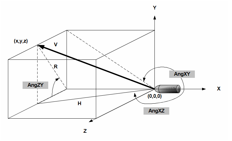
To find a circumferential location of the centre of each fragment, a position of a reference crack is assumed, using a randomly generated number, for each section. The locations of the remaining cracks are then deduced based on values of a_x and a_y. Subsequently, the Cartesian coordinates x,y,z of the initial location of the centre of each fragment can be found. Using the coordinate system indicated in Figure 5, the equations for the point mass trajectory model are:

Figure 5. Layout of strawboard in the trial.

m \frac{d^{2} x}{{dt}^{2}} = - \frac{1}{2} {A ρ C}_{D} V \frac{dx}{dt} m \frac{d^{2} y}{{dt}^{2}} = - \frac{1}{2} {A ρ C}_{D} V \frac{dy}{dt} - m g m \frac{d^{2} z}{{dt}^{2}} = - \frac{1}{2} {A ρ C}_{D} V \frac{dz}{dt}

(3)

where A is the presented area of the fragment taken here as A= a_x.a_y;; $C_{D}$ is the drag coefficient; ( $C_{D}$ =0.91 for subsonic and $C_{D}$ =1.21 for supersonic velocities are used.) $ρ$ is the density of the air; g is the acceleration due to gravity and V is the total instantaneous velocity:

V = \sqrt{({\frac{dx}{dt}}^{2} + {\frac{dy}{dt}}^{2} + {\frac{dz}{dt}}^{2})}

(4)

The initial values of velocity components in the x,y,z directions are obtained from projections and the information about the initial location of the fragment and the projection angle (Figure 6).

Figure 6. Angles used to derive the x,y,z fragment velocity components considered in the 3D trajectory program.

Integration in time, using the three-stage Runge-Kuta scheme, allows the computation of coordinates of the fragment in flight. The ground distribution of fragments can be found by terminating the trajectory at the ground level (for example, for flat ground when y=0). Similarly, when modelling a fragment hitting a target, the trajectory is terminated when the point (x,y,z) enters the domain bounded by the maximum and minimum coordinates defining the target. During the trajectory calculation, it is recommended that smaller time steps are used when the fragment flies in the vicinity of the target.

Results

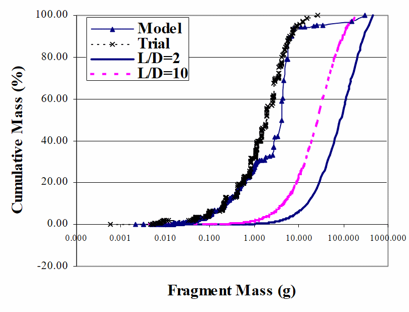
Figure 7 shows the cumulative mass versus fragment mass graph, obtained for a 105-mm shell filled with Composition B explosive. The definition of geometry and experimental results are provided in [15]. The computation is in very good agreement with fragment trial data. For completeness, an alternative approach (by transforming the warhead into a cylinder and then applying Mott’s approximation) is also included to illustrate that it provides a substantially less accurate estimation, even when the length to internal diameter ratio of the cylinder was increased from two to ten.

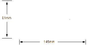
Figure 7. Graph of cumulative mass versus fragment mass; 105-mm (Comp B) shell; from left to right: Trial data; Model prediction; Mott’s approximation indicated as L / D of 2; Model prediction; Mott’s approximation indicated as L / D of 10.

An open-ended half-mortar bomb filled with plastic explosive PE4 which is essentially 88% RDX in a mouldable plastic binder was studied next. The trial data [15] comes from an experiment in which a 81-mm mortar bomb was sawn in half and initiated at the wide end—Figure 8. The model simulates a thin wall of air at both the wide and narrow ends. (The thin wall at both ends coincides with the limit of explosive.) The following input data was used: case mass 1.364 kg; density for cast iron 5370 kg/m³; explosive mass 0.324 kg; explosive density 1434 kg/m³ and the length of filing 0.11 m. (Refer to [16] for detailed geometry coordinates).

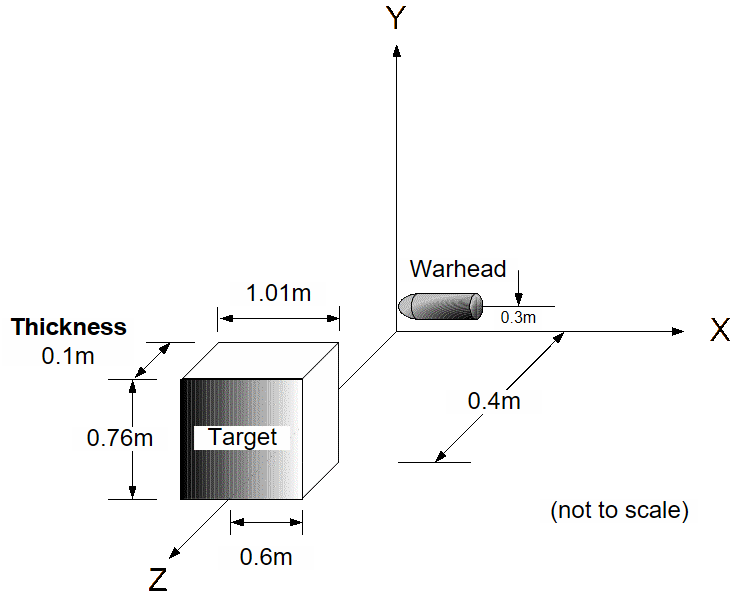
Figure 8. Configurations of the half-mortar bomb.

The strawboard in the trial is located 0.4m from the warhead and measured 0.8m to 1m (Figure 5). The relevant portion is 0.8m × 0.8m and this is simulated in the model as a target. The board consists of twenty strawboards of 5-mm thickness each. Therefore, the total thickness is 0.1m. The ground distribution of the fragments cannot be validated due to a lack of experimental data. However, the vertical distribution on a target face can be matched against the strawboard target of a trial (Figure 9).

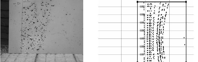
Figure 9. Half-mortar bomb—comparison of fragment distribution on target vertical face. Photograph of the straw board used in the trial (left), and numerical computation (right). Bullet points are used to visualise fragment distribution obtained from the model.

The profiles show a good match. As further validation, the weight and number of fragments collected from the strawboard is compared against that captured in the model—Table 1 and Table 2 respectively—and show a good agreement, noting that not all fragments were recovered during the trials. To aid the comparison, only fragments that weigh more than 0.01g were considered in the simulation, as this was the lowest weight recorded in the trial. In addition, in the trial the secondary fragments discovered in the same hole were disregarded.

In a computation all fragments are accounted for. The fundamental check is to ensure the conservation of mass by simply comparing the initial weight of the shell and the total weight of fragments. Consequently, a model should always result in a prediction of a larger number and total weight of fragments, than it is possible to record in a trial. The accurate recording of smaller fragments is difficult while larger fragments can undergo a secondary fragmentation or can be missed. Other potential sources of error may be an inaccurate specification of the charge and a crude definition of the mortar geometry affecting the angle of the fragment hitting a screen. There are many factors that can influence trial results. Tables 1 and 2 illustrate this. The discrepancies between the two firings are greater than 12% in weight and 26% in the number of fragments. A larger number of smaller fragments was collected in the first firing.

The initial fragment velocity was measured at a point positioned in the middle of the mortar length. The measurement was conducted with a set of pin gauges, a voltage being recorded when the expanding case contacted each pin. The initial separation of case and pin, and the time of contact being known; the expansion velocity was calculated. The oscilloscope trace was noisy and the technique needs refinement but the relevant peaks were analysed. The likely error in the position of the pins is 10%. The averaged from two firings initial velocity is 1167 m/s and the predicted initial velocity from the model [8] is 1086 m/s.

It may be of interest that the initial velocity computed by the model was also compared with results obtained from a modified Gurney’s equation. Such equations are available for simple geometries and in this case a comparison involved a finite cylinder with end-wall on both ends. The relevant modified Gurney’s equation is derived in [6] and provides only the average velocity. The average velocities for the 2.25/1 length/diameter ratio finite cylinder with end-walls were: modified Gurney, 1239m/s; and model, 1200 m/s; and for the 1.3/1 length/diameter 1075 m/s and 1074 m/s respectively.

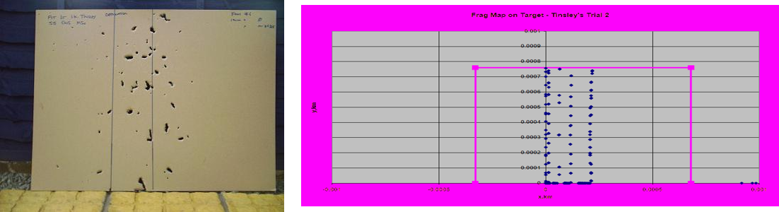
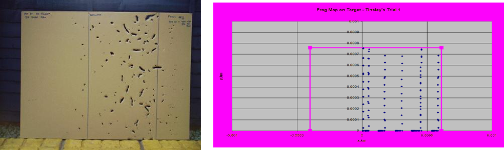
The results obtained for a half mortar bomb proved to be consistent with additional trials using simple geometry pipe bombs, filled with the same explosive as the mortar bomb. For illustration the numbers of fragments obtained from a short cylinder with dimensions: a 130-mm long, open-ended cylinder, with the 50-mm and 64-mm inner and outer diameters respectively, are given in Table 3. Figure 10 shows the corresponding fragment distribution on the target face. Figure 11 illustrates the analogous fragment distribution but for a long cylinder of 9/1 length/diameter ratio for which 109 fragments were collected from the target and 119 computed.

Figure 10. 2/1 length/diameter cylinder—comparison of fragment distribution on target vertical face. Photograph of the straw board used in the trial (left), and numerical computation (right). Bullet points are used to visualise fragment distribution obtained from the model.

Figure 11. 9/1 length/diameter cylinder—comparison of fragment distribution on target vertical face. Photograph of the straw board used in the trial (left), and numerical computation (right). Bullet points are used to visualise fragment distribution obtained from the model.

Table 1. Comparison of fragment weight, collected from the target, in the experimental firing and computed.

1^st Firing	2^nd Firing	Model
51.7 g	57.8 g	68.6 g

Table 2. Comparison of fragment number, collected from the target, in the experimental firing and computed.

1^st Firing	2^nd Firing	Model
104	77	129

Table 3. Comparison of fragment number collected from the target, in the experimental firing of a short cylinder and computed.

1^st Firing	2^nd Firing	3^rd Firing	Model
60	91	57	93

Concluding remarks

The presented methodology is simple, requires easily obtainable, basic input parameters and takes minutes of computation on a personal computer. The speed of computation is relevant as trajectories of over one hundred thousand fragments may need to be modelled for a typical shell. The illustration of the model included in this paper is very limited by sparse availability of the reliable experimental data in open literature. The quantitative comparisons presented here do not reflect the true accuracy of the approach. The more detailed comparisons with classified, high quality arena trials, have been used to verify the model [11]. Nevertheless, the qualitative comparisons with experiments shown in this paper are very good. Further work is required to allow for modelling of non-axial and multipoint initiation.

References

[1] N. Mott, “Fragmentation of Shell Cases”, Proceedings of the Royal Society, 189, 300–15, 1947.

[2] D.E. Grady and M. Kipp, “Geometric Statistics and Dynamic Fragmentation”, J. Appl. Phys, 58, 1210-22, 1985.

[3] L. Zang, X.G. Jin, H.L. He, “Prediction of Fragment Number and Size Distribution in Dynamic Fracture”, J.Phys.D: Appl, 32, 612-615, 1999.

[4] R. Gurney, The Initial Velocities of Fragments from Bombs, Shells and Grenades, BRL Report No 405, Aberdeen Proving Ground, Maryland, ATI 36218, 1943.

[5] T.E. Sterne, A Note on the Initial Velocities of Fragments from Warheads, BRL Report No 648, US Army Ballistic Research Laboratory, Aberdeen Proving Ground, Maryland, 1947.

[6] Extension of Gurney Formulas, Document S5B-4, Honeywell Systems & Research Division, Feb 1965.

[7] D.J.J. Jayaratnam, The Design of High-explosive Fragmentation, PhD Thesis, Royal Military College of Science, Cranfield University, November 2001.

[8] J.Szmelter and C.K. Lee, “Simulation and Measurement of Fragment Velocity in Exploding Shells”, Journal of Battlefield Technology, Vol. 10, No. 2, July 2007.

[9] G.I. Taylor, “Analysis of the Explosion of a Long Cylindrical Bomb Detonated At One End”, in Scientific Papers of G.I. Taylor, 1941, Vol. III, Cambridge University Press 1963.

[10] G. Randers-Perhson, “An Improved Equation for Calculating Projection Angles”, Proceedings of the 2nd International Symposium on Ballistics, Daytona, March 1976.

[11] J. Szmelter et al, Validation of the Natural Fragmentation Methodology, Cranfield University RMCS Report DCMT/ESD/JS/1289/06, 2006.

[12] D.E. Grady, M.M. Hightower, Natural Fragmentation of Exploding Cylinders, Proc. Int. Conf. Shock-wave and high-stain-rate phenomena in materials 713-21,1990.

[13] W. Mock, W. Holt, “Fragmentation Behaviour of armco iron and HF-1 Steel Explosive Filled Cylinders”, Journal of Applied Physics, 54 2344-51, 1983.

[14] J. Szmelter and J.S. Yeo, “A Method for Predicting Natural Fragmentation of Warheads”, Journal of Battlefield Technology, Vol. 6, No. 2, July 2003.

[15] Fragmentation Characteristics and Terminal Effect Data for Surface-to-surface Weapons (U), Joint Munition Effectiveness Manual 61S1-K-UK-3-4, Revision 1, 1 July 1982.

[16] I. Tinsley, Naturally Fragmenting Warhead—An Empirical Method for Measuring Initial Fragment Velocity and an Analysis of Fragment Size, MSc Thesis, Royal Military College of Science, Cranfield University, Jul 2005.

Authors

Dr Joanna Szmelter moved to Loughborough University from Cranfield University (Shrivenham Campus) in October 2006 where she was a senior lecturer in the Ballistics and CFD Group. Prior to this she was in charge of the Aerodynamic Technology Group at BAe Airbus Ltd and earlier she had held various research posts at Swansea University. e-mail: j.szmelter@lboro.ac.uk.

Chung Kiat Lee is a Project Leader in Defence Science and Technology Agency of Singapore. He advises the Singapore Armed Forces in the safety of Explosive Storage and Transport.