Co-Ordination Of Images From Multiple Sensors Into One Common Data Space

Introduction

On the modern battlefield, the use of multiple imaging sensors has a number of significant advantages including the ability to decrease the effect of camouflage and an enemy’s ability to deceive. These images may have been obtained from different platforms, operating at varying orbits or flight profiles, and usually have been taken with a degree of temporal variation. Accurate pixel correlation must therefore be obtained before the images can be fused and credible analysis can be initiated.

To achieve inter-image pixel correlation, subsequent images are geometrically transformed until they match a reference image. This process is sometimes called rubber-sheet transformation, because it may be viewed as a process where an image is “printed” on to a sheet of rubber and then this sheet is stretched and pulled according to some predefined set of rules [1]. The reference points are commonly referred to as control points, which are usually selected around the area of interest to ensure a high level of correlation and accuracy [2]. This is because a rubber-sheet transformation tends to introduce large errors the further away one moves from a control point.

Traditionally, geometric transformations are used on images that have been obtained by looking directly down on the earth. As a result, the polynomial that performs the transformation is of the first order, only altering the rotation, translational shift, and magnification of the image. Higher order polynomials can take into account other imaging variations like tilt, but due to their higher orders, errors occur rapidly as one moves away from a control point.

With the advances in technology in recent years, imaging systems are playing a greater part in all areas of surveillance and reconnaissance. To be detected, an object has to be in contrast with the background. With imaging radar, corner reflections will produce strong returns, while in the 8-12 µm band, vehicles and equipment will contrast against the cooler background of vegetation. If multiple imaging systems are looking at the same area of interest, then these contrasting targets can be used as control points, and a very accurate transformation can be obtained. It can then be possible to link

each imaging system such that a point in space in one field of view can be accurately located in another field of view.

If this process can be performed accurately, and automated, then applications like passive target selection and allocation for weapons systems and submunitions could be achieved. Navigation, using key features and a digitised map, could also be accomplished. Tank commanders could know where each gun system is aimed, and all sensor systems could be integrated into a common imaging battle space.

This paper outlines the operation and demonstrates the utility of automated geometric transformation to develop a common imaging data space.

Image transformations

First order transformations

To understand how a geometric transformation works it is first necessary to investigate the fundamentals of a polynomial transformation. Figure 1 illustrates two sets of four points creating two quadrangles. These two quadrangles are geometrically equal. The one on the left was sketched first, and then it was copied. The copy was then rotated (anticlockwise), reduced in size and then shifted to the right.

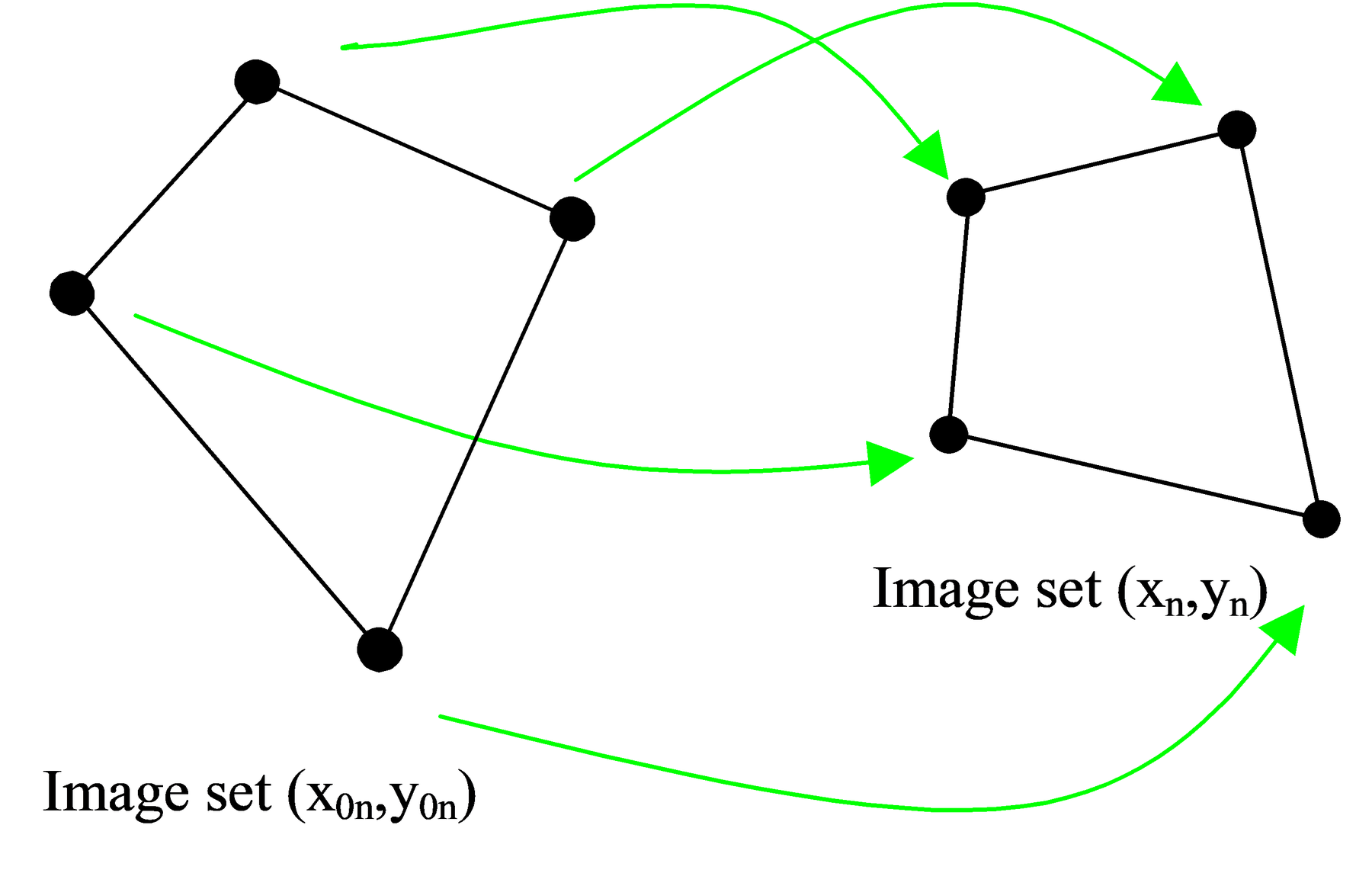
By defining the first image as the Image Set 1 (x_0n,y_0n) and the second as Image Set 2 (x_n,y_n) we can express there relationship as two first-order equations:

$x_1=a_0+a_1{x}_{01}+a_2{y}_{01}$

$y_1=b_0+b_1{x}_{01}+b_2{y}_{01}$

This is a first-order geometric or rubber-sheet transformation. It can be seen that there are three coefficients in each equation. Each coefficient plays a different role in the transformation. The first terms (a₀ and b₀) define the lateral translation in the x-plane and y-plane respectively. This can be simply thought of as an offset. The second terms (a₁ and b₂) control the stretching or magnification of the image, which can have a different value for the x-plane and y-plane. Finally, the last terms (a₂ and b₂) define the rotation of the transformation, by creating an interdependence between the original x, y co-ordinates and the new y, x co-ordinates respectively [3]. This transformation can also be illustrated in matrix form as follows:

$\left|x_1{x}_2\\ x_3\right|=\left|1x_{01}& y_{01}& 1& x_{02}& y_{02}\\ 1& x_{03}& y_{03}\right|•\left|a_0{a}_1\\ a_2\right|$

$\left|y_1{y}_2\\ y_3\right|=\left|1x_{01}& y_{01}& 1& x_{02}& y_{02}\\ 1& x_{03}& y_{03}\right|•\left|b_0{b}_1\\ b_2\right|$

Thus for our previous illustrated example, only three points in each image set are needed to solve for a and b, and thus finding a transformation that correlates each pixel in each image. This type of transformation works well when the area of interested is viewed from above. However, it has limitations when the images are view from side profiles, giving an overall ‘tilt’ to the image set. To overcome this type of limitation, higher-order transformation can be used. Although there is no real limit to the order of the transformation used, only second-order transformations are investigated in this paper, because they provide maximum utility for this type of application.

Second-order transformations

A second-order transformation is similar to the first order transformation described earlier. The simplest second-order equation only has one additional term and is expressed as:

$x_1=a_0+a_1{x}_{01}+a_2{y}_{01}+a_3{x}_{01}{y}_{01}$

$y_1=b_0+b_1{x}_{01}+b_2{y}_{01}+b_3{x}_{01}{y}_{01}$

It is the third term in each equation that determines the amount of tilt to be incorporated into the transformation and can be different for both the x-plane and y-plane. Tilting of an image is also referred to as trapezoidal distorting. By using a grid as a reference image, Figure 2 illustrates the effects of tilt on the original image, in the x and y planes.

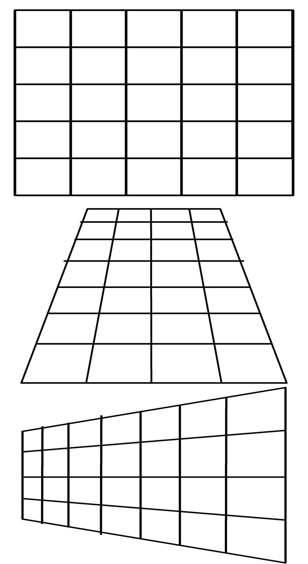
Original Image Trapezoidal Distortion

In Y-Plane

Trapezoidal Distortion In X-Plane

Because of the extra coefficients (a₃ and b₃) contained within this transformation, a minimum of four points, or control points are required to define this transformation. A more complicated second-order transformation contains x² and y² terms. A third-order transformation would contain terms to the power of three. Although these types of terms have very small coefficients, they can cause significant errors the greater the distance from a control point. As a result, the order of the transformation used is selected to match the variations one would predict to be contained with the images to be warped. It is possible to perform a simple second-order transformation using more than four points. This process is known as fitting a least-squares regression solution to the problem. The more points used over the image the more accurate the transformation. This process is not addressed in this paper, and only the simple second-order transformation using four points will be outlined in detail.

The experiment

Scenario and set-up

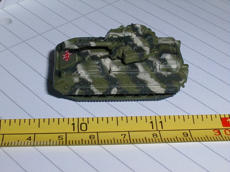
To demonstrate the utility of this image processing system a scenario was developed from which multiple images were obtained. A small board, slightly larger than a door, had been constructed with miniature trees, fake grass and a roadway. Plastic model Bradley Armoured Fighting Vehicles (AFVs) where purchased from a toy store and were measured to be approximately 1:120 scale in size. These were slightly warmed on a heater to assist in developing a contrast in the thermal spectrum. One of these models is illustrated at Figure 3.

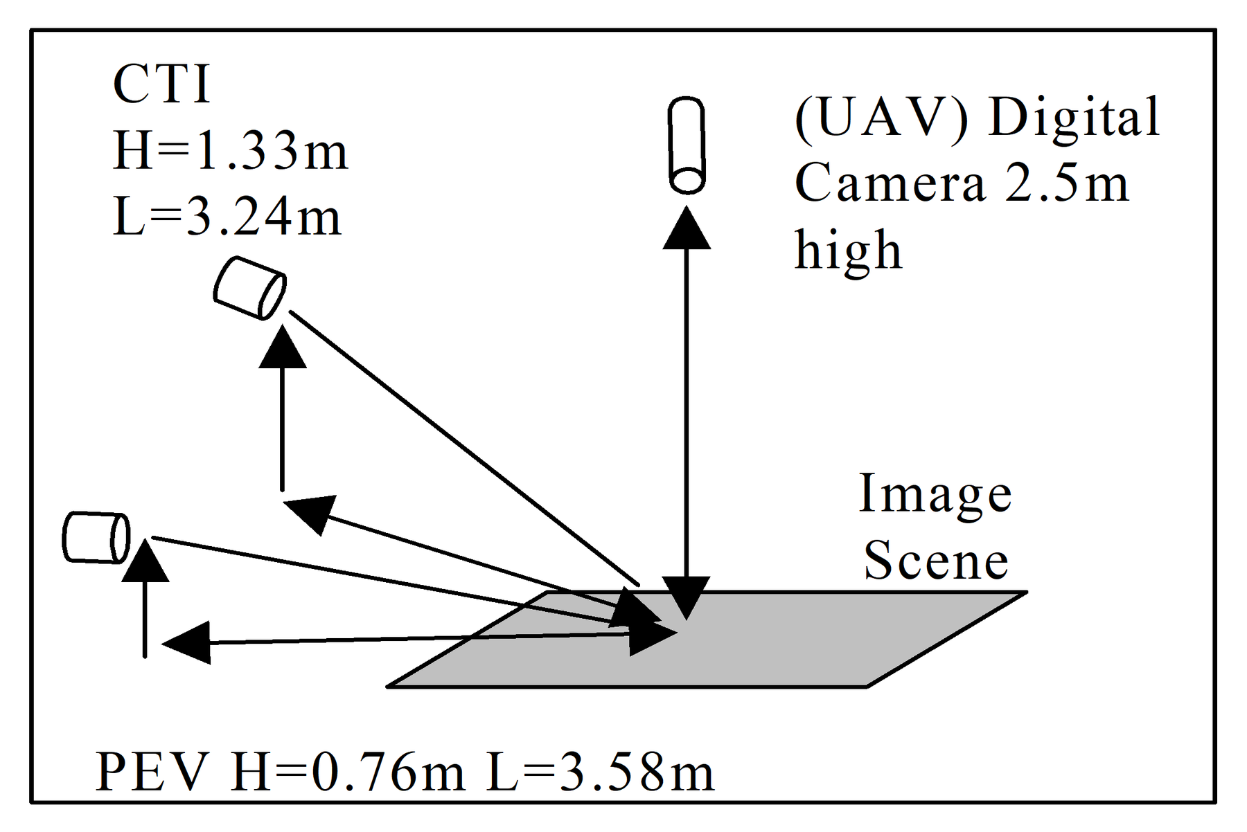
Three imaging systems were used. The first was a Sanyo digital camera, imaging at 1280x960x24-bit colour. Images were taken from 2.5 m directly above the scene, and for this scenario, was playing the role of a UAV loitering above the area of interest. Two thermal images were placed at different points around the board. The first was a Pyro Electric Vidicon (PEV – thermal detector) with an imaging resolution

of 512x360 pixels. It was positioned at a distance of 3.58 m from the centre of the scene and at a height of 0.76 m. The second imager was a Contemporary Thermal Imager (CTI) photon detector with a resolution of 512x512 pixels. It was located at a distance 3.24 m from the centre of the scene and at a height of 1.33 m. The angular distance between the two thermal imagers’ line-of-sight was approximately 50 degrees. The variation in tilt between the UAV image and the PEV image was approximately 65°. The layout of the experiment is illustrated in Figure 4.

A total of eight, slightly warmed, miniature military vehicles were placed onto the scene and a collection of images was obtained. Three of these are illustrated in Figures 5, 6, and 7.

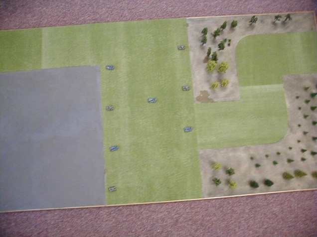
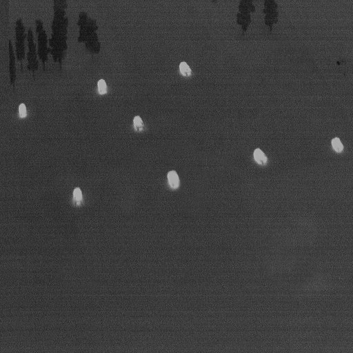
The common features of these three images are the AFVs. If each AFV can be reduced to a point location, and these points assigned corrected to their corresponding points in the other images then a transformation can be found that links each image.

Image preparation

Defining the control points in each image can be performed manually or automatically. To do this manually is quite easy. It is simply a matter of placing a pair of mouse controlled cross hairs over the centre of each AFV and selecting that point. Unfortunately, the exact centre may not always be selected, and human inaccuracies over the whole image may cause a very poor transformation. If this process is automated, then an algorithm may be used to determine the centroid of each AFV. This may be a mathematical compromise between shape and contrast intensity, but this same methodology will be repeated every time, reducing the error of the transformation.

There are a number of steps that must be performed to obtain the centre locations of each AFV. Firstly, the images need to be filtered to remove the noise and to soften the image. This will assist in the location of the strong returns of the AFVs and not a collection of pixels of random high intensities. There are a large number of different techniques and filters that can be used during this process. In many cases, the process used will depend on the imaging platform and the nature of the target’s spectral reflectance. Naturally, it is important to select the tools that maximise the desired output. The best results are produced by filters that erode, but maintain edges, reduce noise, and soften the image. Figures 8 and 9 demonstrate the effects of this process.

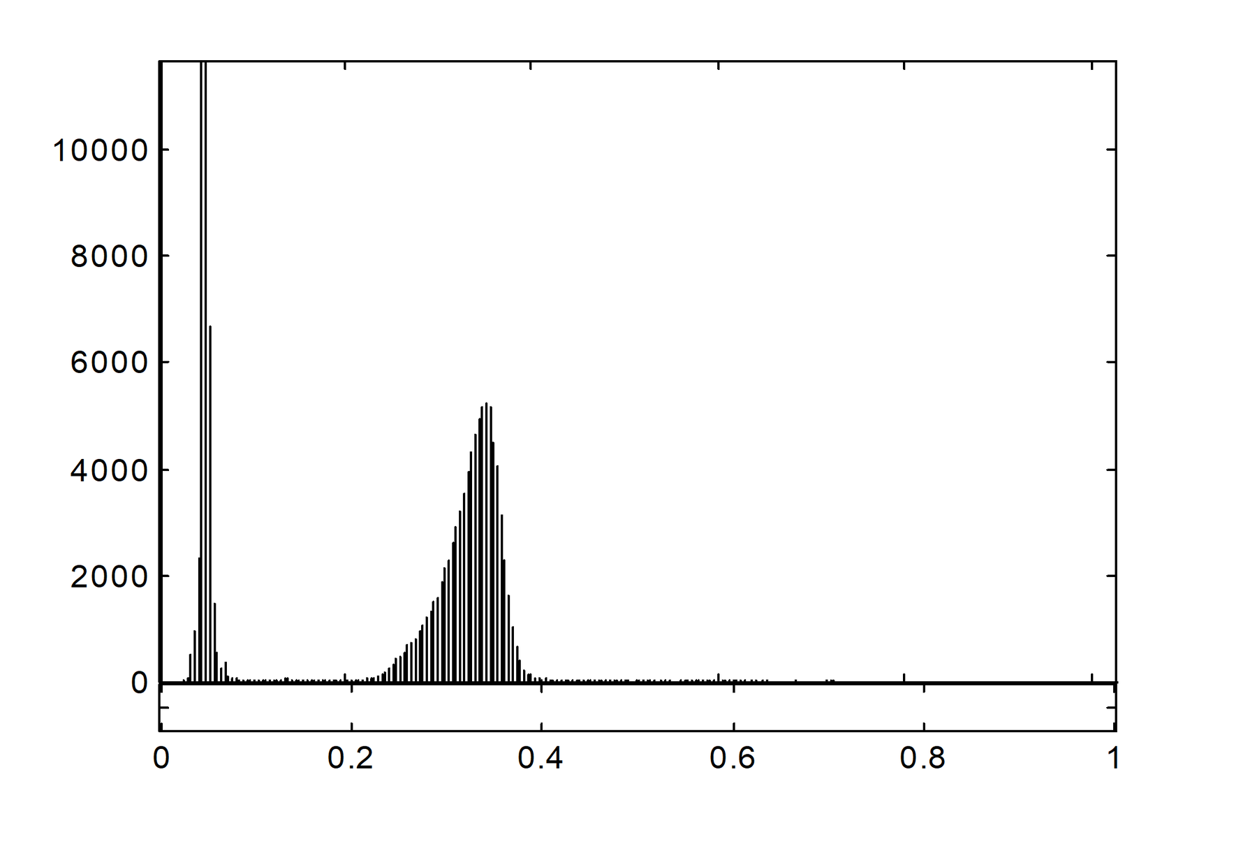
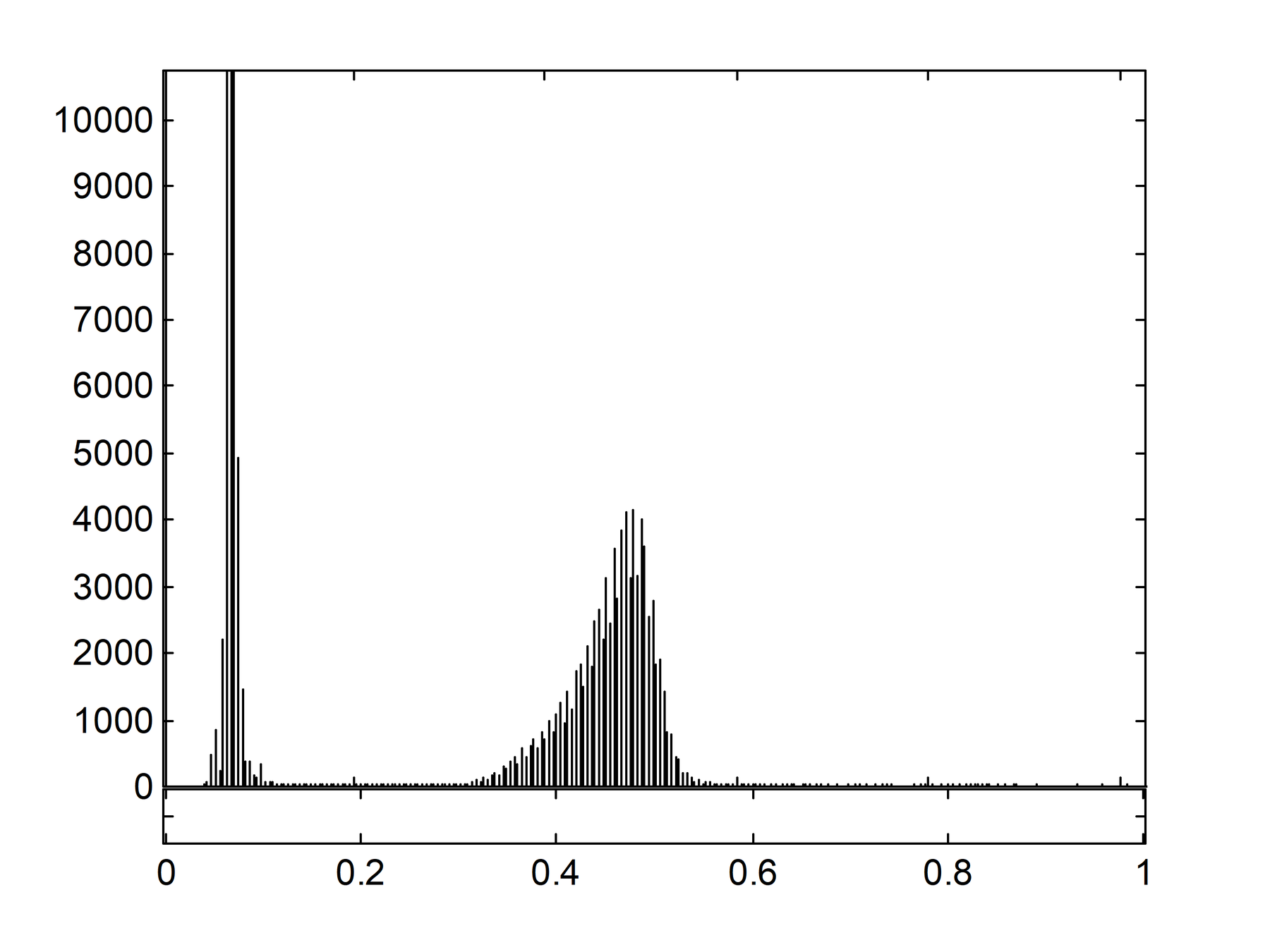
These graphs illustrate the number of pixels in the image for a given value of intensity. The first graph was compiled from the original PEV image data. The second was compiled from the PEV image after the filtering process. It can be seen that the number of pixels with higher intensities has been reduced in the filtered image. Also the population of higher intensities has been shifted to the right. This makes the process of applying a threshold to the image much simpler.

The aim of setting a threshold is to set all pixels below a specific level to black, and the remaining pixels to white. This would be ideal if we were only interested in finding the geometric centre of each target. This technique, however, fails to take advantage of the thermal signature of the targets. It can be assumed that the hottest part of the target will be in the same location on the target regardless of the orientation of the observer, within reason. Thus, to ensure that this information is not lost, only the lower threshold is set to black. The pixels above this threshold are left unchanged. The result of this process for the PEV image can be seen at Figure 10.

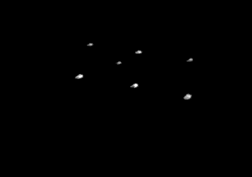
The next step in this process is to locate the centre of each of the remaining pixel groups. A process that takes into account the intensity levels of the pixel as well as the geometric shape will guarantee that the point found will closely match those in other images. If only the geometric shape is used, then this may lead to poor correlation in other images if the target (AFV) is not symmetrical in all three dimensions (like a cube or a sphere). To overcome this, a filter with a gradient can be used, which returns a high value when located centrally and amongst high intensities. The filter used was 25 by 25 cells in size, as illustrated in Figure 11. The outer perimeter was unitary and each side increased in value exponentially as one moves towards the centre.

This filter was shifted about each group of pixels and all pixels were multiplied by the corresponding cell value in the filter. The 625 cells were then added to produce a single value. The filter was shifted about the target until the highest value for that area was obtained. This location corresponded to the centre of the target. This process was repeated through the image set and all subsequent image sets.

This process produces two arrays per image containing x-plane locations and y-plane locations of the centre of each hot AFVs, producing a total of six arrays. To ensure that a nontrivial solution to the transformation is obtained, each point must now be matched to its corresponding point in each image.

Control point selection and allocation

The accurate selection and allocation of control points determines the accuracy of the warp. If the control points chosen are too close together, then the warp will have heavy degradation throughout the rest of the image. If the selected control points are greatly dispersed, then the accuracy in the centre of the image will be poor. A median must be found. It is best to select control points that surround the area of interest. In our case, the area of interest are in fact the control points, so an even distribution vertically and horizontally is required.

Because four points are needed to perform the transformation, the other points in the image can be used to confirm if the transformation is accurate. If one point in one image transforms to a point within the other image to an accuracy of +/- five pixels, then this is a solution. By varying the level of accuracy we can have some control over which control points are selected. It is important not to set too small an error otherwise a warp will not be found. In a similar way, if the error is too large, then trivial solutions may result.

The transformation

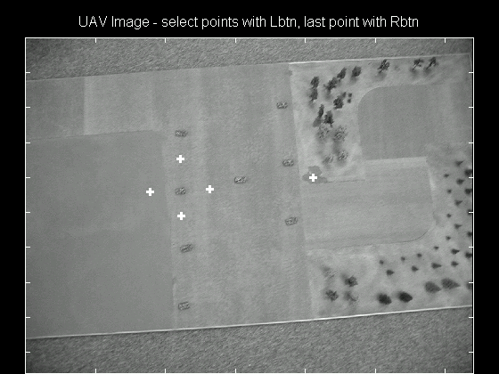
Once the control points have been correctly allocated to the corresponding control points in each image, simple matrix manipulation to solve for a and b, will define the transformation to be used. This will allow pixel-to-pixel interrogation between each image. To illustrate this, five small crosses were marked on the UAV image, and only using the transformations, their corresponding locations were plotting on the two thermal images. The results are illustrated in Figures 12, 13 and 14.

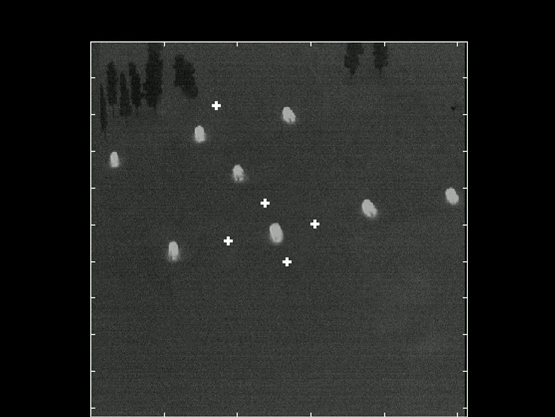
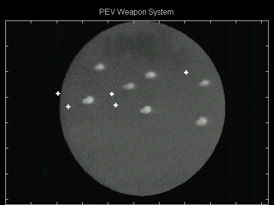
Considering the automated process; four points had to be selected from eight (CTI), which then had to be compared with four points selected from seven (PEV). This totalled 1411200 possible combinations. Although a large number of these combinations would have been acceptable solutions, only 576 of these would have given an accuracy of +/- ten pixels or less. Clearly, to go through all of these combinations and test each one to see if it is a solution takes a considerable amount of processing. Also, there is no guarantee as to when one of the 576 combinations will be found. As a result, for this process to work in real time a powerful processor and a small number of points is required.

It is interesting to note that a pixel that is not within the PEV field of view can still be plotted accurately, as seen in Figure 14. This technique of linking images sets to a common image space using polynomial transformation has a variety of applications. Some of these applications include; navigating by features, passive target designation for submunitions or a salvo of weapon systems, and command and control of weapon platforms for the co-ordination and concentration of firepower.

It is at this point that a comparison between the original image and a warped image would be of some benefit in the assistance of overall comprehension. To illustrate this, every pixel within the CTI image was warped to match the UAV image. These two images were then overlaid to produce Figure 15.

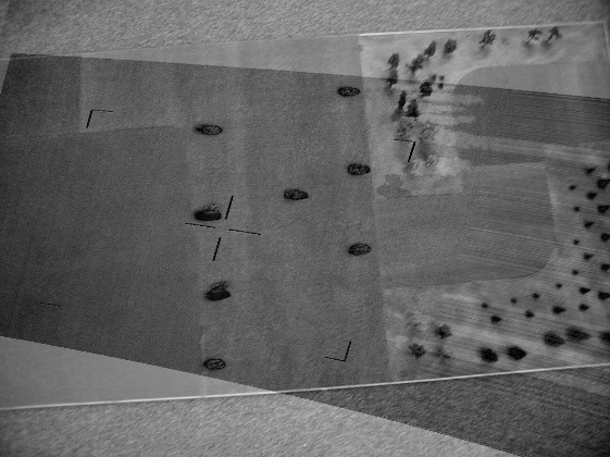
The cross hairs that can be seen are from the original CTI image, that were removed prior to the filtering process. The streaks that can be seen on the right of the image are due to the absence of image data. As a result the program filled to the right of the image with the last pixel value used for that line.

Applications

As mentioned earlier there are a number of applications where this process can be utilised. The first of these is to navigate by features.

For the example outlined above, the features used to transform the images were emissions from simulated AFVs. There is no reason why these features could not have been colder objects such as rivers and lakes, or warm features like a road or tarmac. In fact, any object that is in contrast with the surrounding can act as a control point. This could allow a digital map to be loaded into a system, and the imaging system could follow its position on the map by working out its location with respect to the features it can detect. This could prove to be a very accurate and robust passive positioning system.

The experiment illustrated the utility in using the position of thermal targets to transform different image sets. This technique could allow submunitions to be pre-programmed with a reconnaissance image or even the dispensing systems image. This would be an effective method of allocating a target to each submunition. Because the process uses control points to transform a third-party image into its own image, decoys like flares would allow even more accurate pixel correlation and improve inter-image accuracy.

Finally, as a command and control tool, this process could allow a tank commander the ability to see where each tank under his command has it main weapons system targeted. This would allow maximum delivery of ordnance during an engagement, as targets that are not being aimed at would be instantly identified allowing maximum concentration of firepower through directed control. This would also apply to the gun systems of attack helicopters, and other weapons platforms with imaging capabilities.

Conclusion

It has been shown that images varying significantly with regards to aspect orientation can accurately be transformed

into a common image data space if four common points can be located. Additionally, if there are more than four common features or points, then this process can be automated, and the accuracy improved dramatically.

Many consideration must be made when preparing the images to extract the control points, especially when determining the centre of a collection of pixels to be represented as a single value for x and y.

There are many applications for this type of image field transformation. As computers become more powerful and much smaller, then their ability to handle real time transformations will become practicable. When this is the case, it is the real time application of this process that will deliver the greatest utility to the user.

References

Authors

Captain Vince Polito is currently studying an MSc in Guided Weapons Systems at the Royal Military College of Science in Shrivenham, England. He is a graduate of the Australia Defence Force Academy, where he studied electrical engineering and is an officer in the Royal Australian Electrical Mechanical Engineering Corps. On completion of his MSc he will return to Australia where he will fill the appointment of Guided Weapons Officer for Project Air 87 – Armed Reconnaissance Helicopter Project in the Defence Acquisitions Organisation (DAO). He can be contacted at polito2000@hotmail.com.

Ian Luckraft has degrees from Oxford University and the University of Hertfordshire. He is a lecturer in the Electro-Optics Group at RMCS where he specialises in digital image processing.

References

[1] R. Gonzalez and R. Woods, Digital Image Processing, Addison Wesley, 1992.
[2] R. Schowengerdt, Techniques for Image Processing and Classification in Remote Sensing, Academic Press, 1983.
[3] J. Russ, The Image Processing Handbook, CRC Press, 1994.