Synthetic Aperture Radar (SAR)

Introduction

In the field of airborne reconnaissance, it would a great advantage to have a radar available that could produce a high resolution picture of the ground and provide detailed information about troop movements, building works, railhead activities, and so. This sort of information can of course be obtained by photographic imaging infra-red techniques. These, however, require the reconnaissance aircraft to at best fly near, and at worst fly over, the ground of interest. An imaging radar, on the other hand, could achieve the same result at a large stand-off range by using its superior atmospheric attenuation properties, and its relative immunity to weather effects. This paper deals with the theory and practice of such radars.

In order to achieve high-resolution pictures of the ground, it is necessary to achieve high resolution along the radar beam (range resolution), and across the beam (cross-range resolution). High range resolution is achieved by the use of pulse compression – a technique that is not discussed further in this paper. Cross-range resolution is a function of antenna beamwidth and target range. High cross-range resolution, therefore, is achieved by producing a radar antenna with a very narrow effective beamwidth. To achieve this, a real antenna would have to be made impracticably large. The solution is to find some way of synthesising the performance of a very large antenna out of one that is physically far smaller. A technique for doing this is described below.

Formation of a synthetic array

The beamwidth (θ_B) of a real antenna is given by:

${\theta }_B=\lambda /D$

where D is the antenna width, and λ is the wavelength of operation. This gives a cross-range resolution, δ_cr, of:

${\delta }_{cr}=R\lambda /D$

where R is the target range. High cross-range resolution therefore requires very large antennas – normally impracticable on most realistic platforms.

Figure 1 illustrates the production of a synthetic array, where the motion of the platform is utilised during transmission of the ranging pulses to give an effectively long antenna – a so-called synthetic aperture.

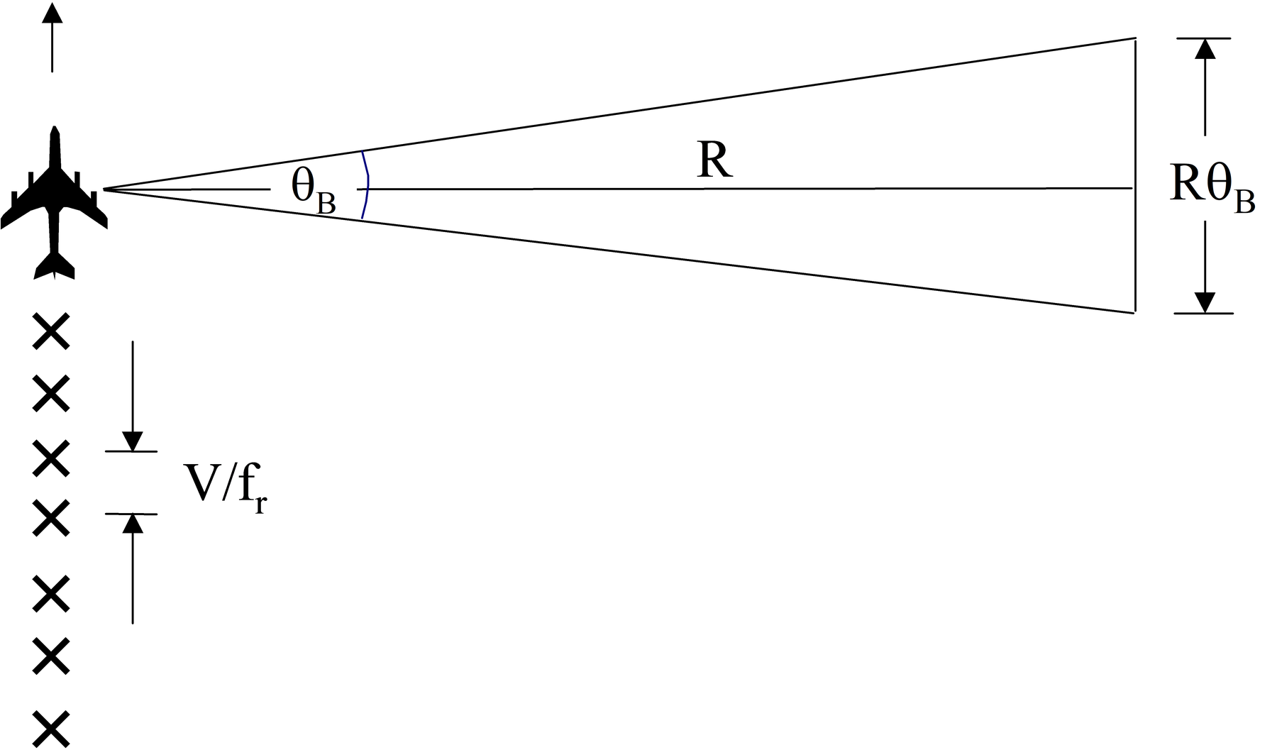
The aircraft is flying a constant velocity (V), sending out pulses (at frequency f_r) at 90º to the flight line. Each pulse is sent from a different location on the flight line, and defines one element of the synthetic array. The total array consists of all positions at which an echo is received from a particular target. All the echoes from this target are then processed to form the synthetic array beam pattern. The beamwidth of the array is given by:

${\theta }_s=\lambda /2L_e$

where L_e is the effective length of the synthetic array. (This differs from a real array beamwidth by a factor of two. This is because synthetic array beamwidths are determined by a two-way phase pattern, while real arrays use a one-way pattern.)

The cross-range resolution available from the synthetic array is thus given by:

${\delta }_{cr}=R\lambda /2L_e$

The effective length of the array is determined by the distance along the flight line over which a particular target is in the beam of the real antenna. This given by:

$L_e=R{\theta }_B$

and is a function of target range, being longer for more distant targets. Since θ_B=λ/D, the cross-range resolution is:

${\delta }_{cr}=D/2$

which is independent of range.

Thus a synthetic array is capable of resolving cross-range detail down to half the size of the real antenna, regardless of range! Because array patterns are produced by adding the element contributions taking account of phase, and because the synthetic array has stored these contributions over a period of time before combining them, the approach outlined here is sometimes known as the phase history approach.

Angular resolution improvement using doppler frequency history

An alternative, but entirely equivalent, approach to the one above is the frequency history approach. This utilises the fact that the echoes from a particular target undergo a Doppler frequency sweep as that target travels through the real beam. This Doppler frequency is positive as the target enters the beam, falls to zero when the target is exactly abeam of the aircraft track, and then becomes increasingly negative until the target passes out of the back edge of the beam. A Doppler filter centred on zero will only accept targets that are abeam of the aircraft track, eliminating all others. Thus we have achieved cross-range resolution by the use of frequency discrimination. This approach is illustrated in Figure 2.

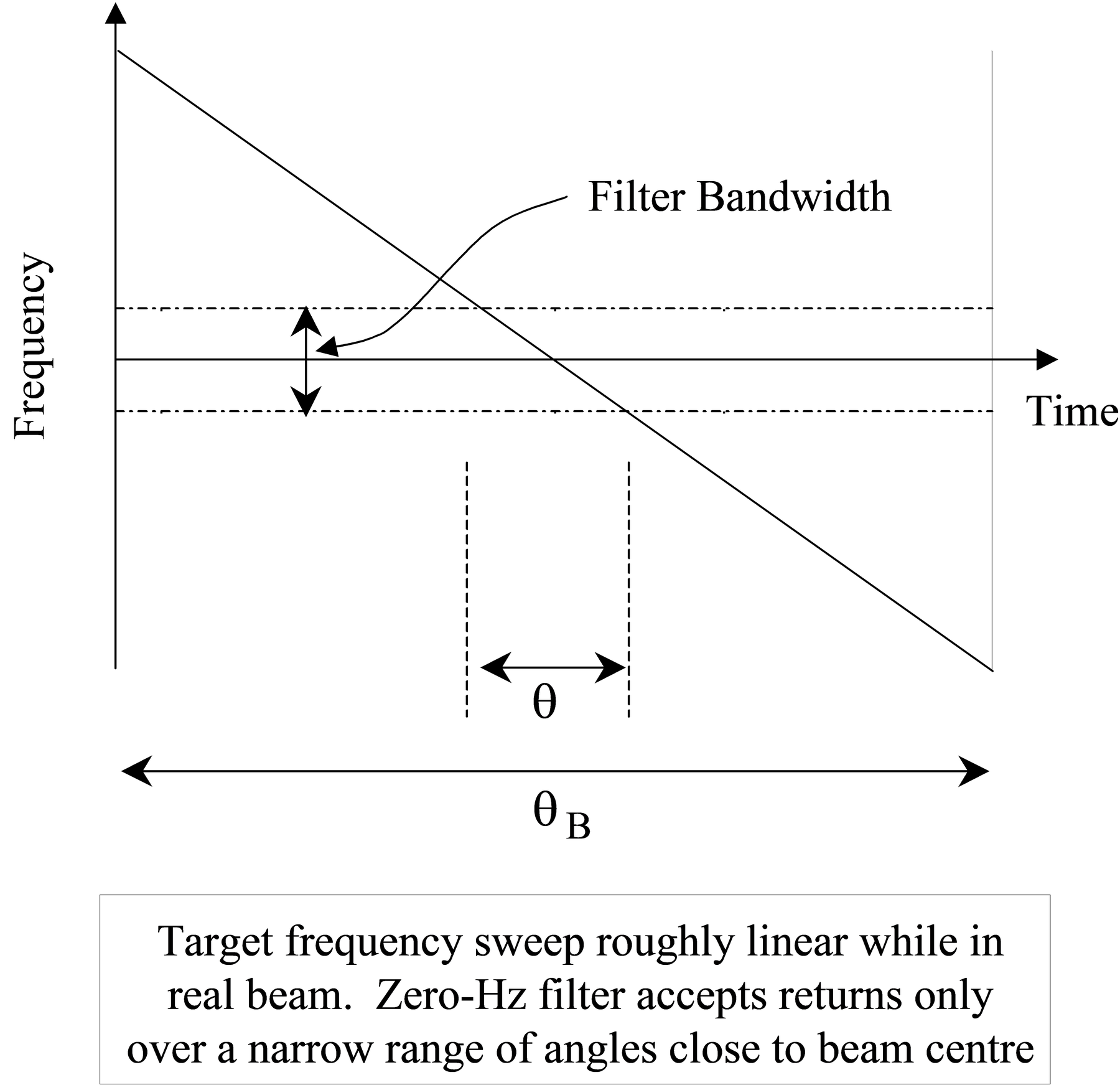
The cross-range resolution of the system is limited by the minimum bandwidth that can be achieved by the filter. This is given by:

$\Delta f=1/t_{int}$

where t_int is the filter integration time. This is limited to the length of time that echo power is being returned to the radar receiver. This is the time that the target is illuminated by the real beam:

${tB}_{int}$

where V is the aircraft velocity, and θ_B is small enough to make it equal to its sine. Hence the range of Doppler frequencies accepted by a filter tuned to zero Hz will be:

$+V/2R{\theta }_B\text{to -V/2R}{\theta }_B$

But for a particular target θ/2 off the aircraft beam direction, the Doppler frequency of a returning echo is given by:

$f_d=2V\mathrm{𝑠𝑖𝑛}(\theta /2)/\lambda$

In order to enter the filter, targets must have values of θ/2 constrained by the expression:

$2V\theta /2\lambda \le \text{V/2R}{\theta }_B$

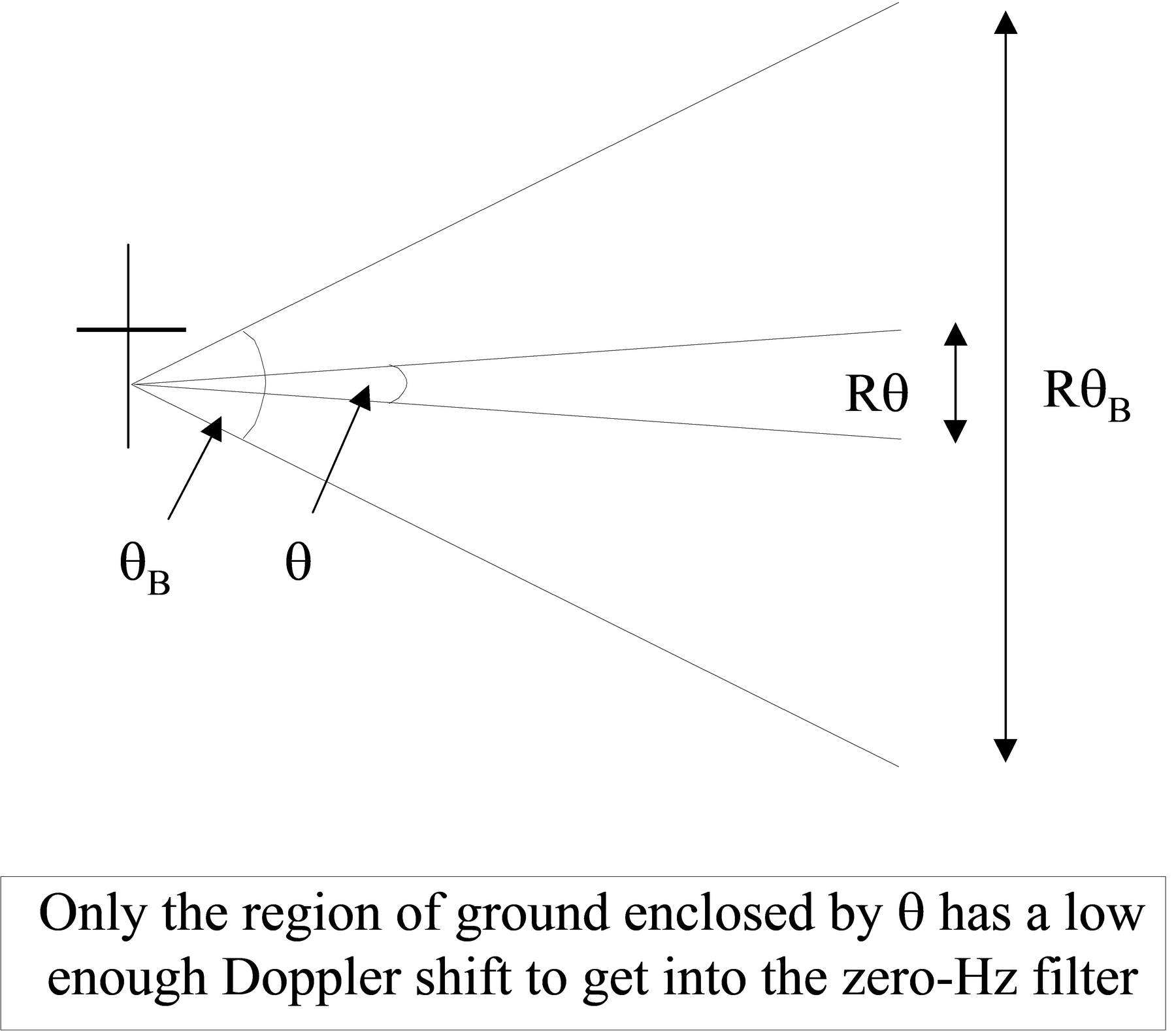
assuming that θ is small enough to equal its sine. Noting that the cross-range resolution is Rθ, and the real antenna beamwidth is θ_B=λ/D, this reduces to:

${\delta }_{cr}=D/2$

This is the same result that was obtained earlier using phase history, and is illustrated in Figure 3.

Unfocused and focused arrays

Normal array theory assumes that the target is far enough away to treat the incoming signal as a plane wave. This implies a straight wave front and hence, when the target is at right angles to the line of the array, all element contributions are in phase. This effectively means that it is assumed that the array is focused at infinity. For a real array, this is a perfectly reasonable assumption, because the target distance is always much larger than the array length. For synthetic arrays, however, this is not true, because as the target gets further away, so the array gets longer. Thus one is always dealing with a curved wave front, and even in the centre of the main beam there are path length differences (and hence phase differences) between the elements of a synthetic array. Once the end elements are more than 90º out of phase with the centre elements, these element contributions start to subtract from the phasor sum, and the gain of the array starts to fall. This increases the beamwidth and reduces the resolution of the array. (This is precisely the same phenomenon as is experienced when using an optical instrument focused at infinity, and trying to look at objects much closer to you. The image is blurred, and detail is lost.)

There are two ways to combat this problem:

Limiting the length of the array. This approach leaves the array unfocused, but limits the length of the array to those elements that are no more than 90º out phase with the middle. Figure 4 shows the geometry of this. Using Pythagoras’ Theorem, it is easy to show that the array length is limited to (Rλ)^½, and so the cross-range resolution is given by:

${\delta }_{cr}=(R\lambda {)}^{1/2}/2$

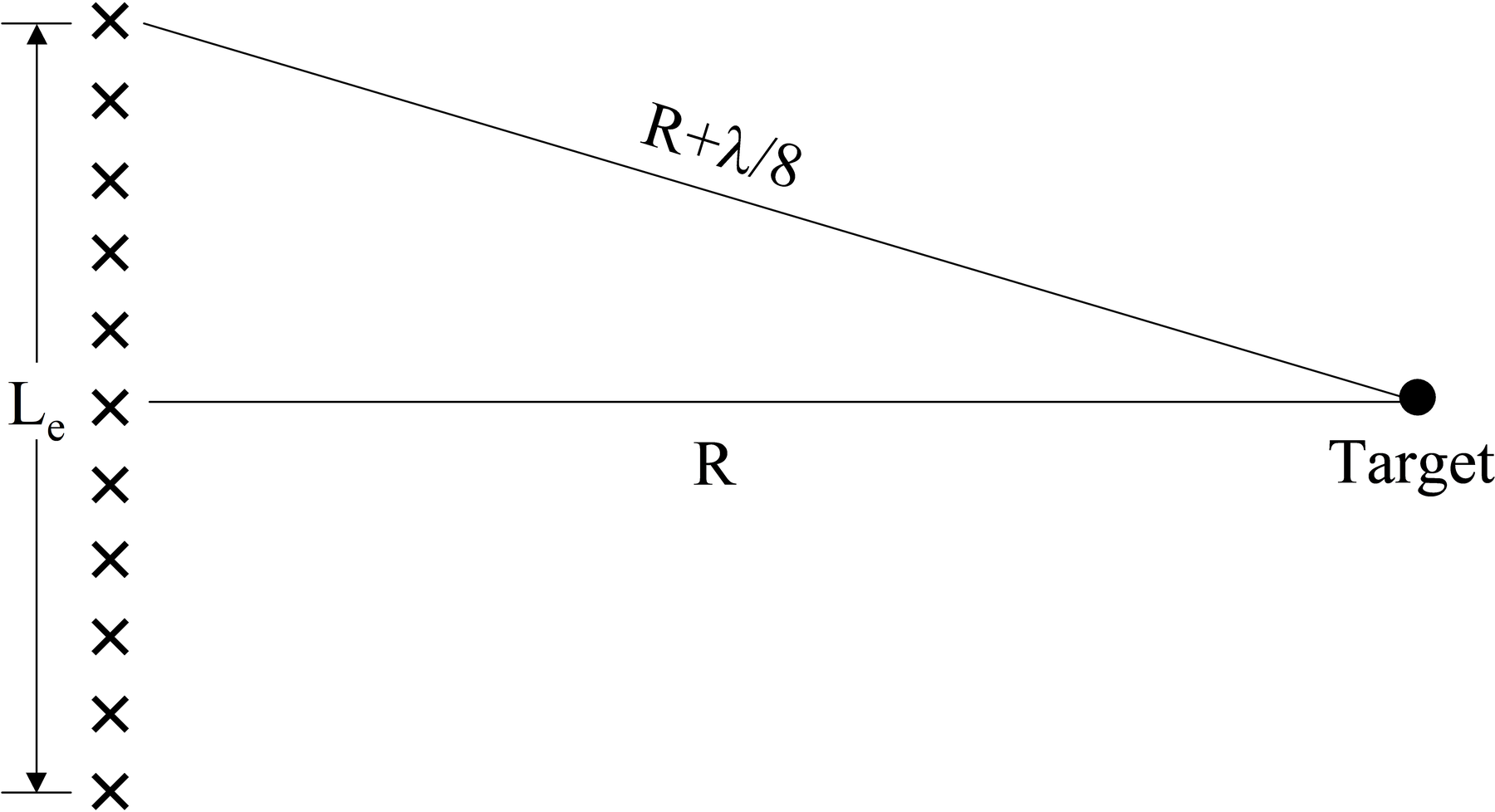
This approach is quite easy to implement, requiring very little processing. Consequently it was adopted in some early systems. However, the cross-range resolution is now range-dependent and while it still much better than the real antenna, it represents a deterioration in performance which increases with range. It is desirable to do better.

Correcting the phase. This approach calculates the phase corrections needed to bring boresight echoes into phase at all elements. This approach effectively focuses the array to the range of a particular target. In practice there is a different set of corrections for each range, and hence the amount of processing can be colossal, with a separate set of corrections for each range-cross-range resolution cell.

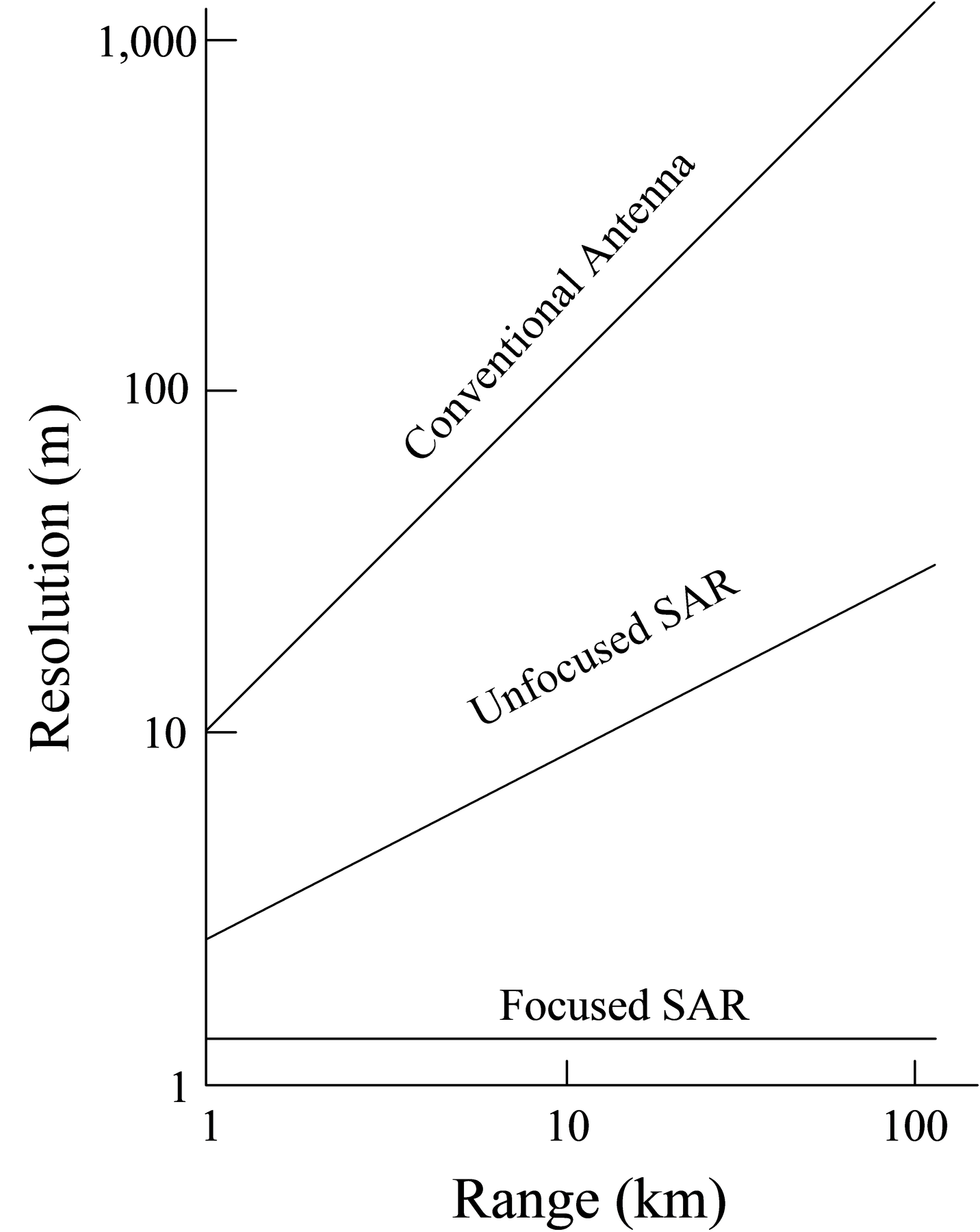
Despite the immense amount of processing involved, it is the focused system that is used almost universally nowadays. Consequently this is the approach discussed further in this paper. However, for reference, Figure 5 shows the cross-range resolution as a function of range for focused, unfocused, and real arrays.

Grating lobes, PRF and swath width

As illustrated in Figure 6, if the elements of the synthetic array are laid down with too large a spacing, grating lobes appear, giving angle ambiguity for the target.

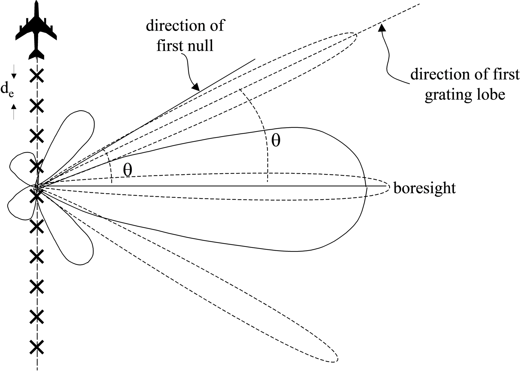
This can be avoided if the angle, θ_g, between the first grating lobe of the synthesised array and the beam centre is greater than the angle, θ_n, between the first null of the real antenna pattern and the beam centre. That is:

${\theta }_g>{\theta }_n$

where θ_n, is given by:

${\theta }_n=\lambda /D$

and θ_g, is given by:

${\theta }_g=\lambda /2d_e$

where d_e is the element spacing. The element spacing in turn is given by:

$d_e=V/f_r$

All of this leads to the condition:

$f_r>2V/D(=V/{\delta }_{cr})$

Thus the requirement on the position of the grating lobe leads to minimum PRF. PRF determines the maximum unambiguous range (R_mu). Thus there is a link between δ_cr and R_mu, which can be determined by substituting for f_r in the above equation to obtain:

$R_{mu}/{\delta }_{cr}<c/2V$

Figure 7 illustrates the limitation this places on the coverage of the system.

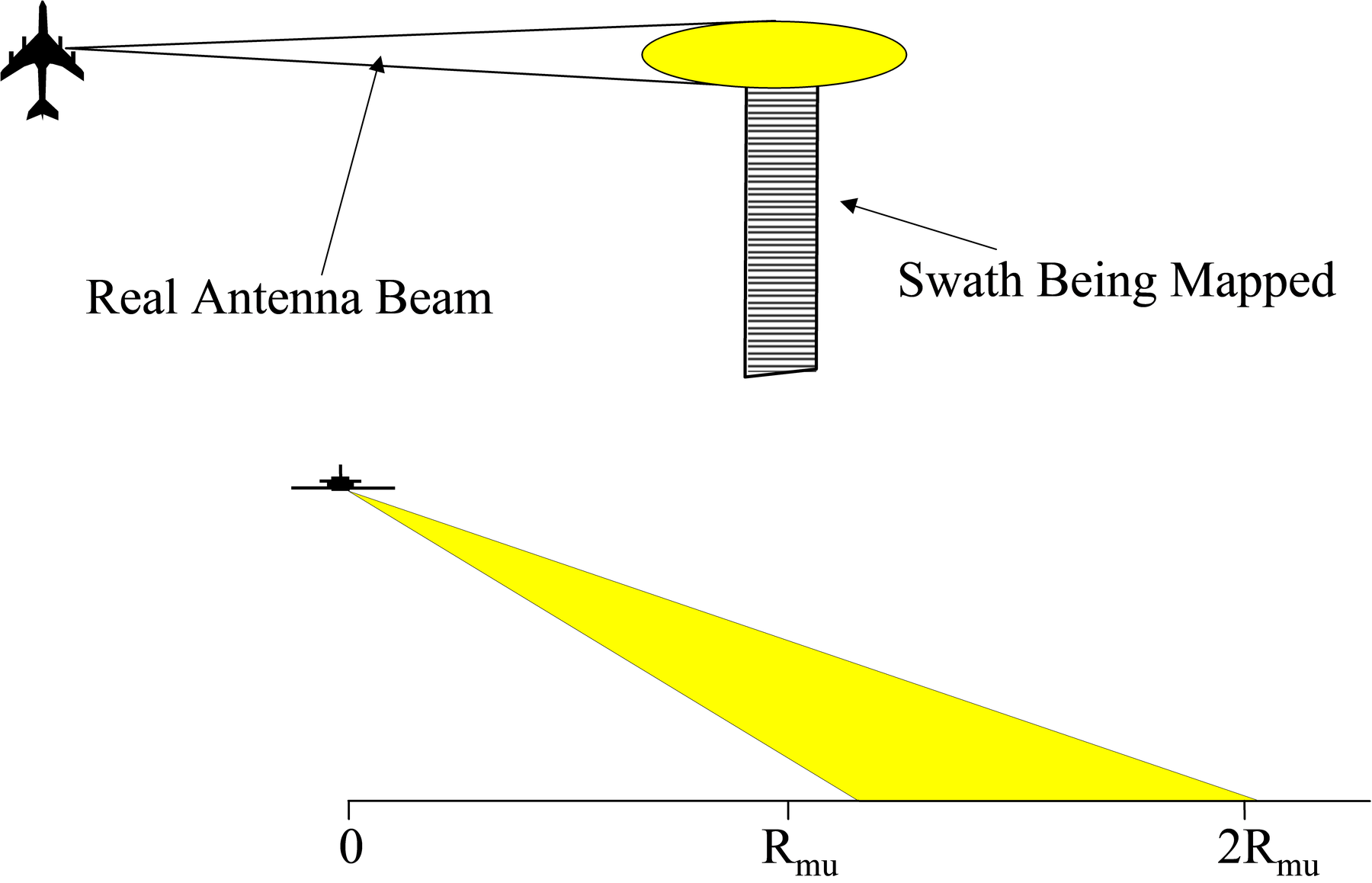
It can be seen that as the platform travels, it can only deal with a swath of ground from the minimum range observable in the vertical beamwidth of the real antenna to a range R_mu greater than this.

Doppler-cross-range coupling and motion compensation

Up to this point, it has been assumed that all frequency and phase variations have been produced by the steady motion of the platform past the target. There are two ways in which this assumption can be violated.

• Target Motion. If the target has an inherent Doppler shift, this will superimposed on the frequency history of that target, causing the timing of the its appearance in the zero Doppler filter to be affected. Thus a cross-range error will be introduced. This is known as Doppler-cross-range coupling. Using the phase history approach, the Doppler shift will cause a progressive phase error in the element contributions, and this will cause the processing to mis-position the array centre, and hence the position of the target in cross-range. Whichever way you look at it, the result is the same - moving targets are misplaced in azimuth. Targets that change their motion during the dwell time of the real beam will have a variable cross-range error. This causes blurring, and thus a loss of cross-range resolution. There is little that can be done about this problem in any of its forms.
• Irregularities in Platform Motion. In practice, aircraft do not fly absolutely steadily. Air turbulence causes the flight path to be irregular both in line and in speed. This will cause blurring of the target in both range and cross-range, for reasons identical to those given above. However, now there is something that can be done. Irregularities in platform motion can be monitored, and suitable corrections made to data being processed. The current way of achieving this is to take the output from the Inertial Navigation system, and use this information to compensate for irregularities of motion. This technique is known as motion compensation. Prior to the use of motion compensation, most SAR work was done from space, where motion irregularities do not exist to the same extent.

The processing used in image production

Thus far, the principles behind high-resolution radar have been discussed. This section discusses the process of producing the high-resolution map from the radar data. These days this is done digitally, and uses either unfocused processing or focused processing. Of these, unfocused processing involves the least computation, and has been used for a quite a long time. Focused processing required much more capacity, and was beyond the capabilities of near-real-time computing until relatively recently.

Both methods start the same way. The radar sends a pulse out through the real antenna and, during the inter-pulse period, receives returning echoes from all points on the ground that are illuminated by the real beam. Different ranges give different echo times, so the total echo is spread out in time according to range. This echo is mixed coherently with the transmitted waveform to produce a video signal that contains the amplitude and phase of all returns in the real beam, sequenced in order of increasing range. This signal, which represents the returns for one element in the synthetic array, is stored. Another pulse is sent, and the procedure is repeated, thus laying down the echoes for the next array element. This process continues, with the returns for each element being stored. Once enough element returns have been accumulated, it is now possible to combine the return from a given range for all the elements, thus synthesising the array to produce high resolution in cross-range. It is how this process of combining is done that distinguishes the two processing methods. (In each case pulse compression is used to obtain the required resolution in range.)

Unfocused processing

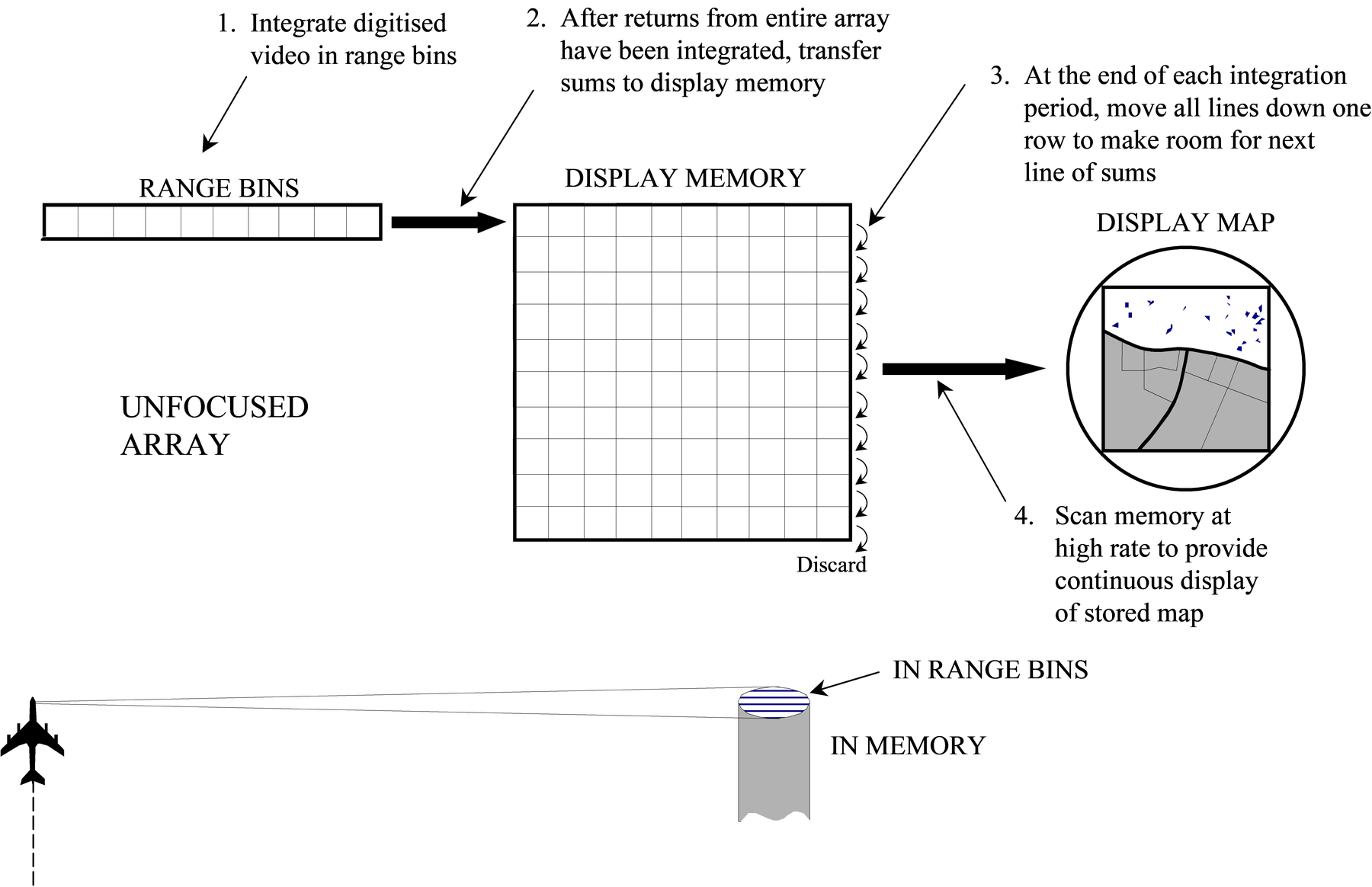
In unfocused processing the video signal from the returning echoes is divided into range bins, and digitised to retain amplitude and phase information. The returns from the first pulse are stored in appropriate range bins. The returns from successive pulses are added into these range bins. This is the process of integration that is familiar in simple pulse radar. However, here the returns will only add to give a large amplitude if they are all in phase. This will only happen if the target is at 90º to the flight line of the aircraft. All other returns show a progressive phase shift from pulse to pulse, and integration will not give a large answer. Since this process favours targets on the beam of the aircraft and suppresses all others, a narrow array beam has been synthesised. (This process is identical to that involved in a real array, which also forms its narrow beam by adding all element contributions taking account of phase to form a narrow beam.) When a pre-determined number of elements have been integrated, the result is passed on to a display memory, which uses the information to produce one line of the image. The integration then starts again. Each time the display memory gets one line of data, it moves all older lines down its store by one line. Thus it is able to display the image all time to include the latest processed information. Figure 8 summarises this procedure.

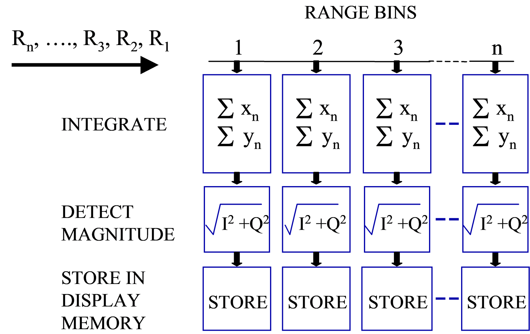
The computer procedure involved is illustrated in Figure 9.

Notice that phase information is retained by processing both I and Q channels, and then squaring and summing. This removes the problem of blind phase, and gives a correct value of echo amplitude.

The approach outlined above is straightforward, and in near real time. In practice, there are two complications:

The synthesised array takes no account of phase errors (that is, it is not focused). It is therefore limited in length, as has been discussed earlier.

As it has been described here, the array is the same length for all ranges. This makes the storage problem easy. If one wished to synthesise an array of different length for different range, it can be done. It does involve storing each pulse separately, however, and operating the integration for a given display line over a different number of stored returns for each range bin. Since the integration can only take place after all the relevant returns are in, the display line cannot be formed until the data for the longest range bin is ready. In practice, the complications outweigh the advantages.

Focused processing

With advances in the speed and capacity of modern computers, it has become possible to focus an array digitally in reasonable times. The processing is summarised in Figure 10.

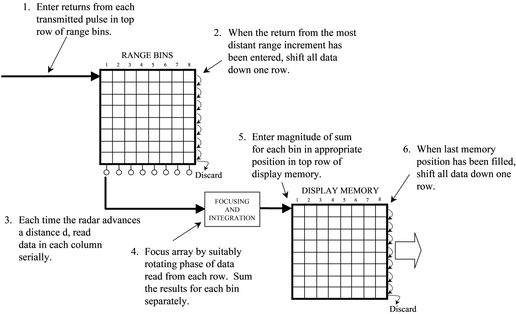
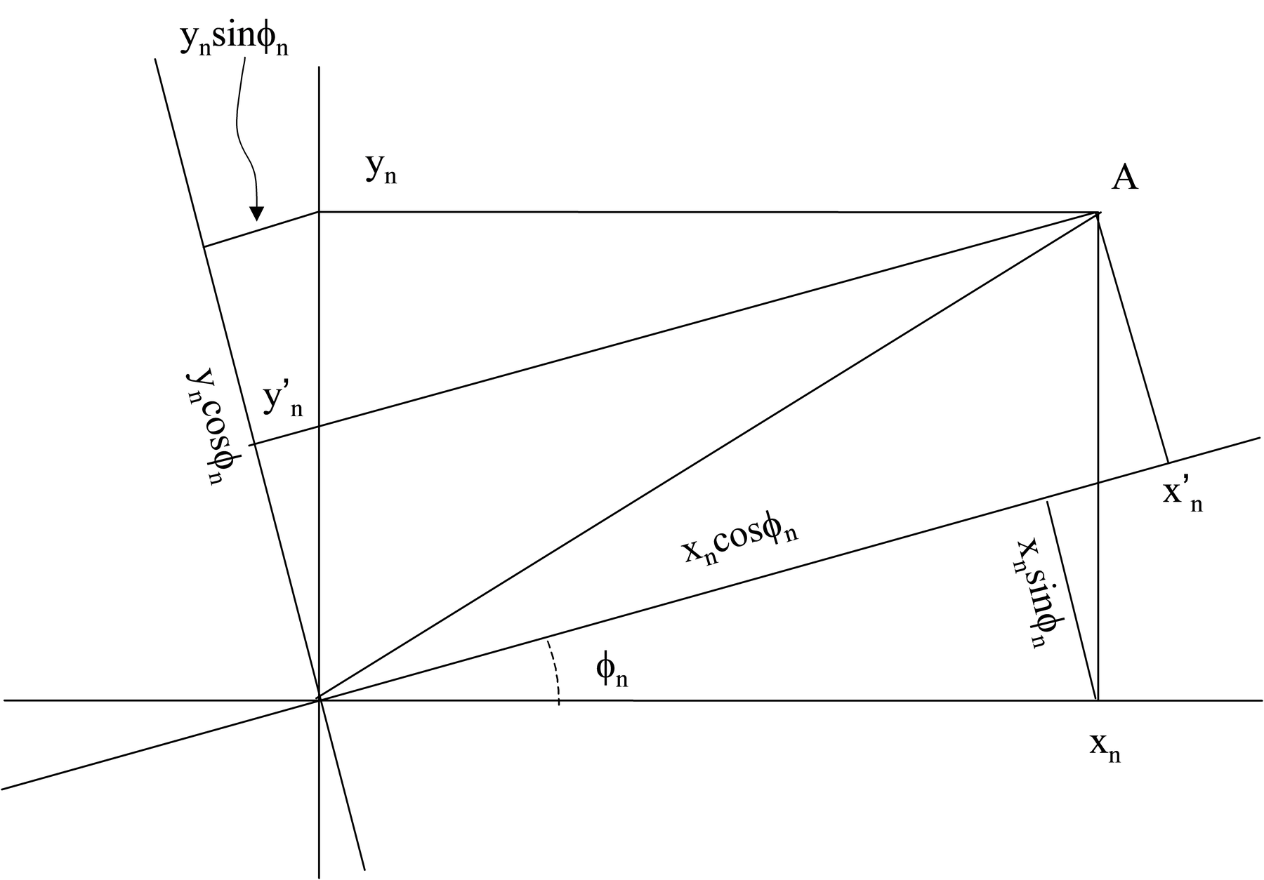
A two-dimensional store of signal history is used, consisting of digitised returns arranged in range bins and array elements. Focusing involves correcting the phase digitally for a sequence of element returns for a given range bin. Each phase correction is equivalent to a co-ordinate rotational transformation as illustrated in Figure 11.

The I and Q components of the phasor before rotation are x_n and y_n. After rotation, new I and Q components x’_n and y’_n are given by:

$x{\text{'}}_n=x_n\mathrm{𝑐𝑜𝑠}{\phi }_n+y_n\mathrm{𝑠𝑖𝑛}{\phi }_n$

and:

$y{\text{'}}_n=y_n\mathrm{𝑐𝑜𝑠}{\phi }_n-x_n\mathrm{𝑠𝑖𝑛}{\phi }_n$

Integration of the corrected I and Q components for the entire range bin is now carried out:

$X=\Sigma x_n^{\text{'}}and\text{Y}=\mathrm{\Sigma }{y}_n^{\text{'}}$

and the magnitude of the phasor sum can be obtained from:

$S=\sqrt{X^2+Y^2}$

The corrections for a given range bin are always the same, thus this process can be repeated line by line. Different range bins require different corrections, but this causes complexity rather than difficulty. The above computations are identical to those involved in forming a digital filter by DFT.

The major problem with this line-by-line approach is the mass of computing involved. Each time the radar sends a pulse, it gets another set of data, and one can produce another line. This means that each time the radar moves one element along its track, an entirely new array is synthesised. This involves a completely new set of phase corrections in each range bin, for each pulse. Clearly, much capacity is needed. There are four operational solutions:

• Reduce the resolution by synthesising smaller arrays, and producing fewer display lines. This approach currently allows near real-time operation. In practice it also tends to produce resolution that deteriorates with range.
• Concentrate on a small area of ground that is of particular interest, and process this to full resolution. The computing load is reduced by ignoring other areas.
• Data link the raw data down to the ground, and do high resolution processing there. This method is not in real time.
• Use Doppler processing instead of array synthesis. This method allows parallel processing of lines, and also enables the use of FFT techniques.

The first three of the above are self-explanatory; the fourth is discussed in somewhat greater detail below.

Doppler processing

Figure 12 shows the frequency history of five points all at the same range but spaced evenly in cross-range, and Figure 13 shows an enlarged version of the detail enclosed in the rectangle.

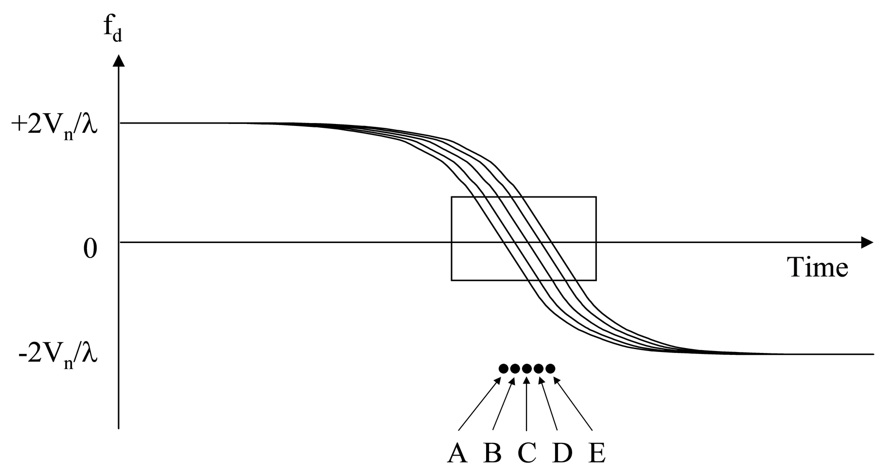
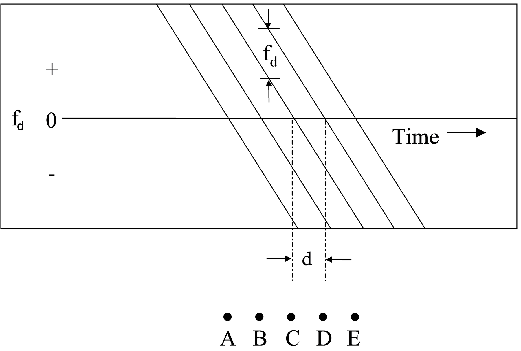
Although all five histories are the same shape, they cross the zero-Doppler line (that is, they are precisely abeam of the aircraft) at different moments. This causes frequency differences between the returns. This allows separation of the returns via Doppler filtering. The method is straightforward, consisting of two basic steps:

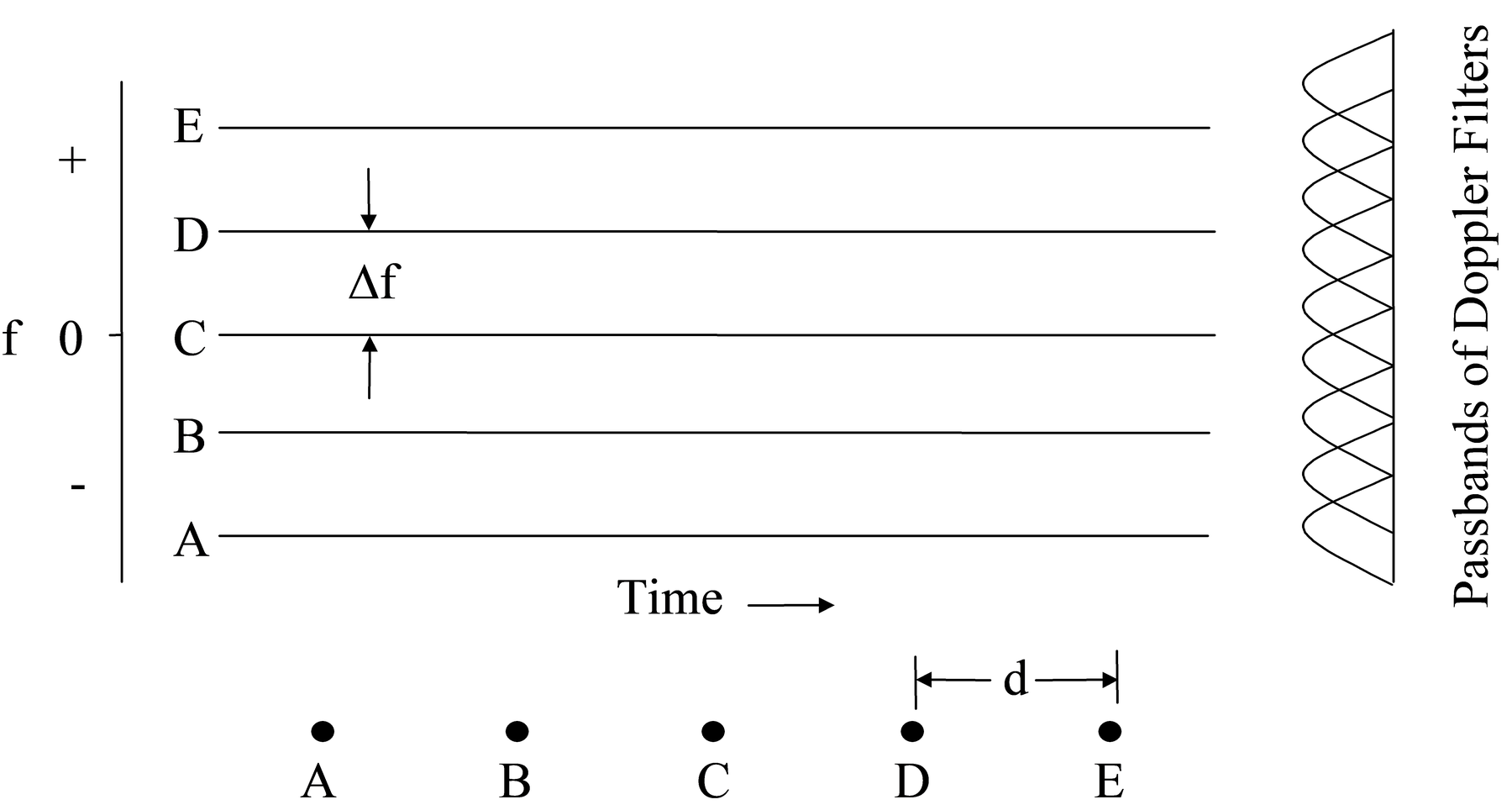
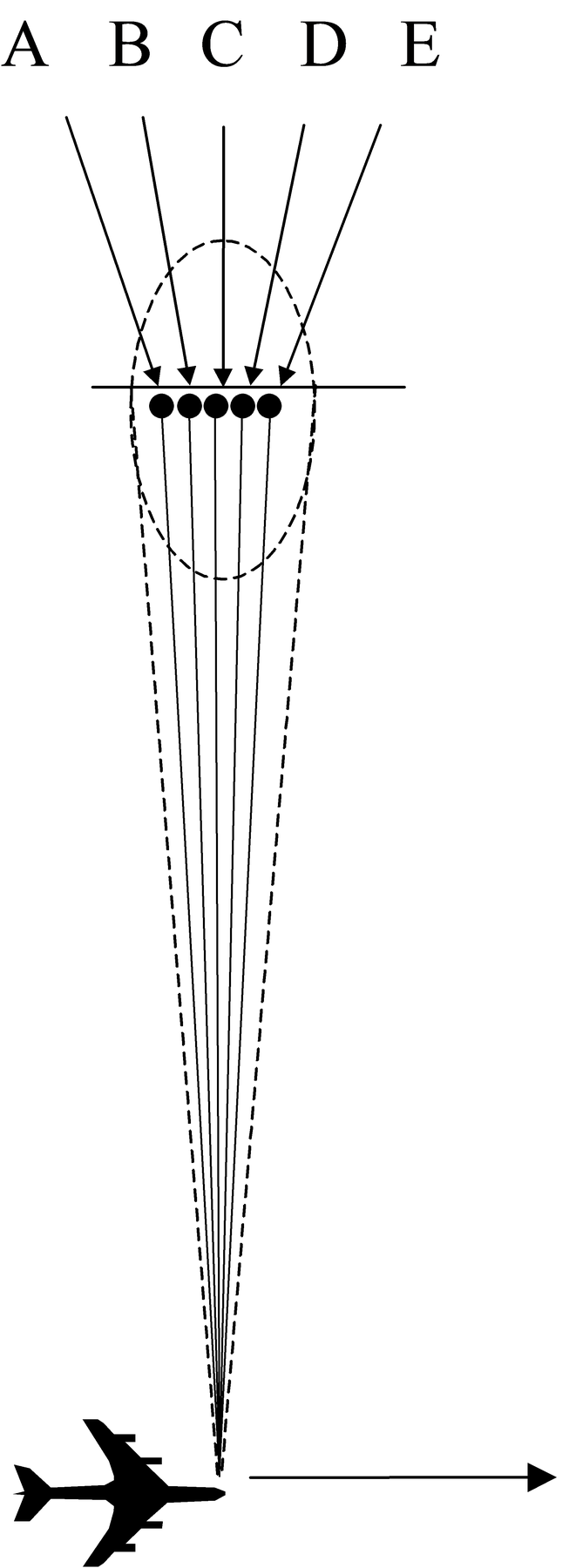
Focusing. The returns are corrected in phase. This has the effect of removing the frequency sweep. However, the frequency differences mentioned for the five targets are preserved through this process, and appear as five constant frequencies, one for each target, as illustrated in Figure 14. The value of the frequency is indicative of its cross-range position. Thus target location as illustrated in Figure 15, may be obtained by measurement of this frequency. This can be done with a suitable filter bank. The implementation of such a bank is outlined below.

Range Gating and Doppler Filtering. After focusing, the returns are range-gated and stored. Then, for each range bin, a Doppler filter bank is generated from an appropriate set of returns. Figure 16 illustrates the scheme.

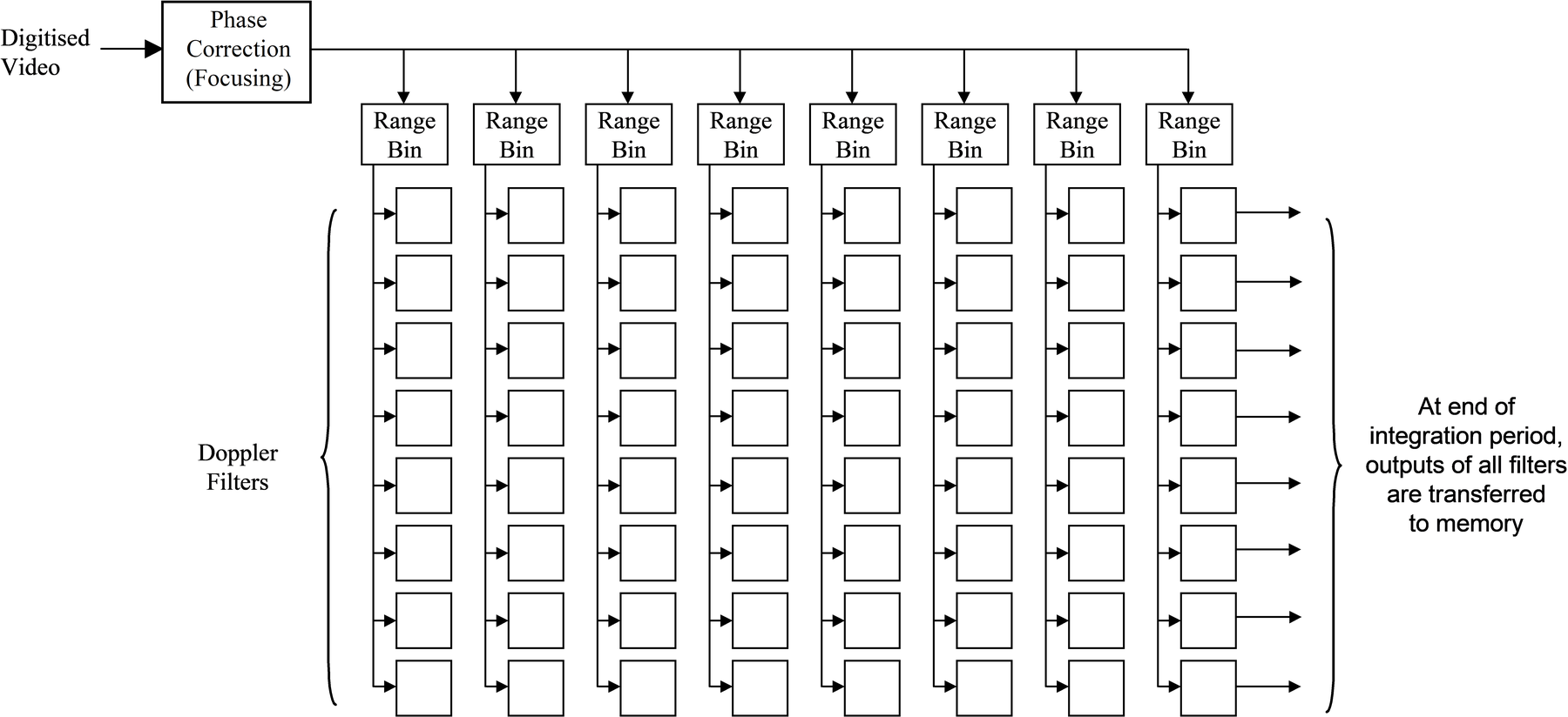
If the number of returns processed is a power of two, and the number of filters in the bank is the same power of two, then FFT techniques may be used to cut down the amount of computing required. However, the gains are greater than that. Each filter accepts the echo for a particular frequency. But that particular frequency is a function of cross-range position of the target. Thus each filter is, in effect, processing one point for the final displayed image, and the whole filter bank is processing a number of display lines at a time. This is parallel processing, and hence the production of the final image is very much faster. Also, the phase corrections involved in focusing (which are so processing intensive in the line-by-line approach) need only be done once for each set of processed lines instead of once for each line. Figure 17 illustrates both line-by-line and parallel processing in terms of the production of scan lines in the swath image.

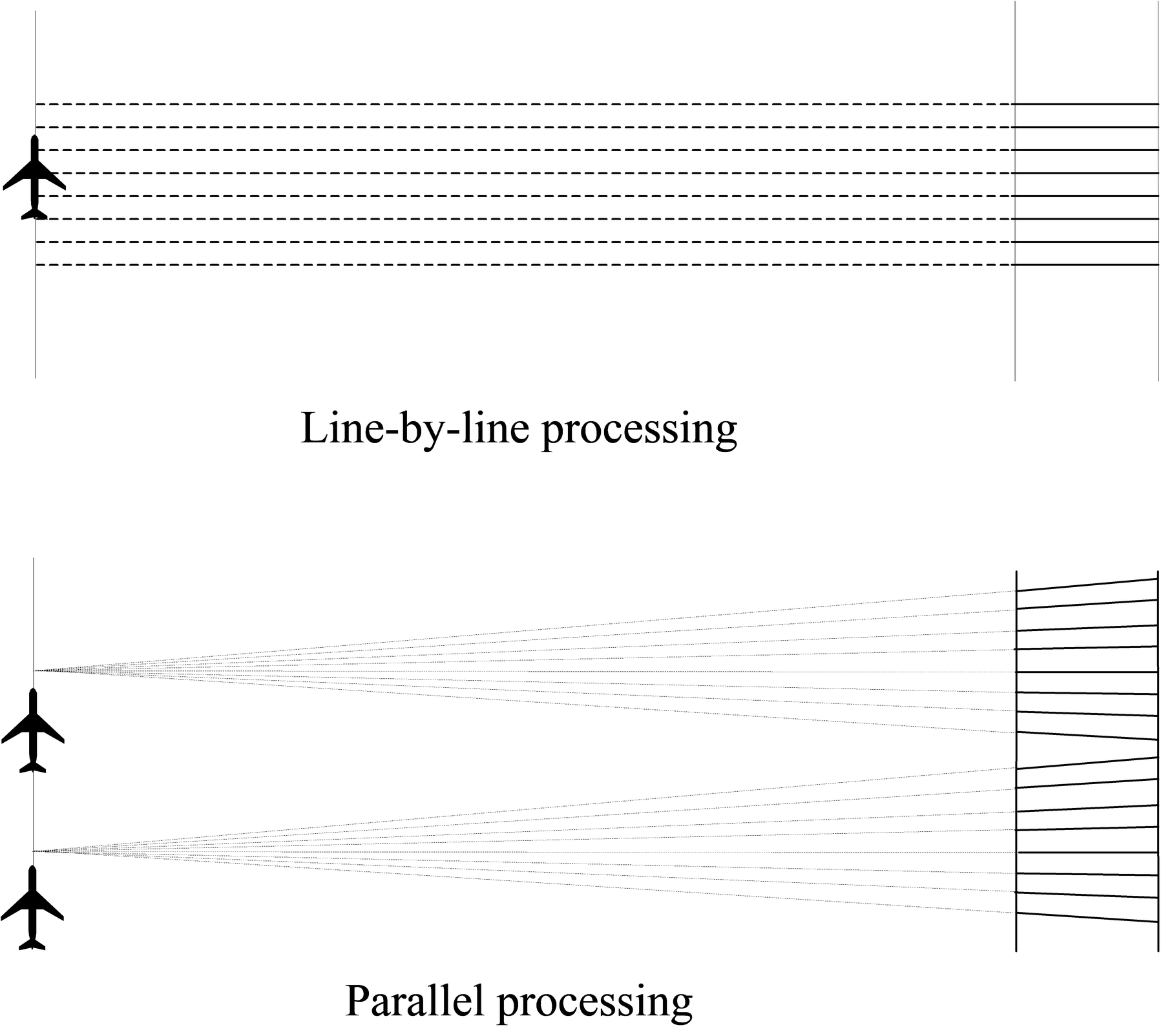
Notice that parallel processing produces scan lines that are not quite parallel. This leads to a slight distortion in the image. In practice, however, the swath is usually small compared with the range, and so this effect is usually negligible.

Beam steering

The discussion on Doppler processing has shown that it is possible to process imagery that is not abeam of the aircraft by simply using a filter that is tuned to some frequency other than zero. Actually, the beam of the synthetic array can be steered in exactly the same way as a real array (that is, by adding in a progressive phase shift along the array). The advantages and penalties of this are identical for a synthetic array. The principle one of interest here is the broadening of the array beamwidth as the steering angle increases. In synthetic arrays, this has the effect of worsening the cross-range resolution. The beamwidth of a steered array in terms of the unsteered beamwidth is given by:

$\theta ={\theta }_B/\mathrm{𝑐𝑜𝑠}{\theta }_s$

By complementary angles, this is equivalent to saying that the steered beamwidth, and hence the cross-range resolution, degrades as the sine of the angle to the flight line decreases. However, accepting this resolution loss, beam steering allows three operational approaches of advantage.

Forward steering

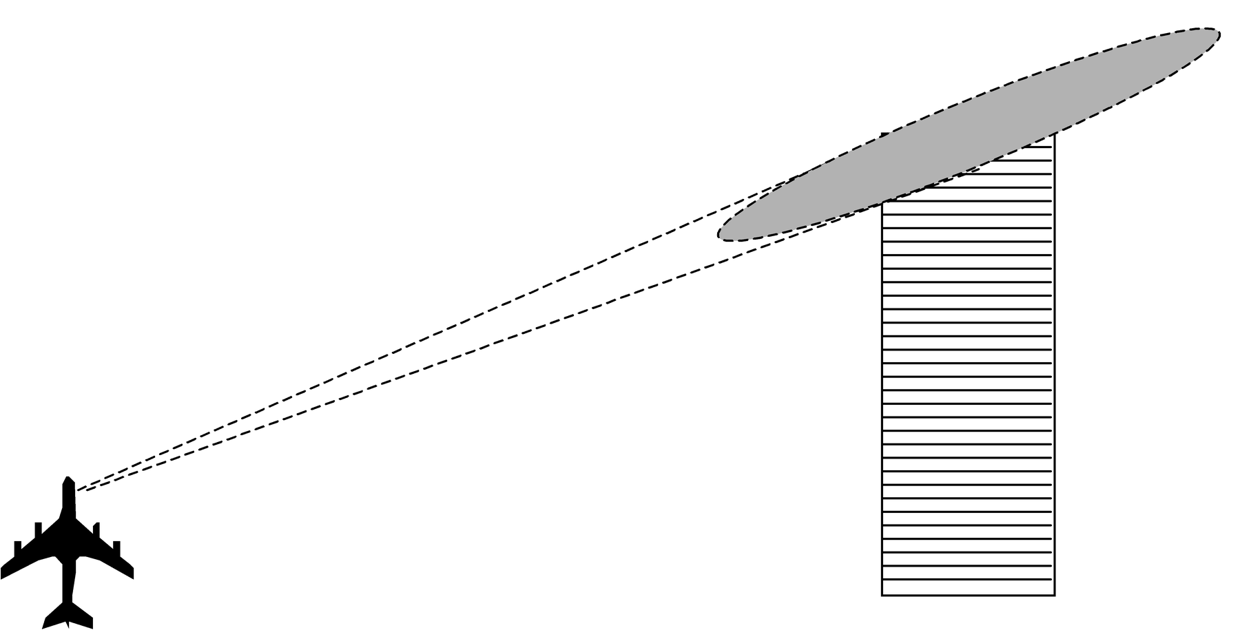
One problem with conventional side-looking SAR is the fact that one has already passed the ground that one is imaging. This was no problem when the processing was slow. Now that the processing can be done in real time, however, it would be nice to see the ground that one has not yet reached. By steering the beam somewhat forward of the abeam direction, this is achievable. Figure 18 illustrates the idea.

Doppler Beam Sharpening

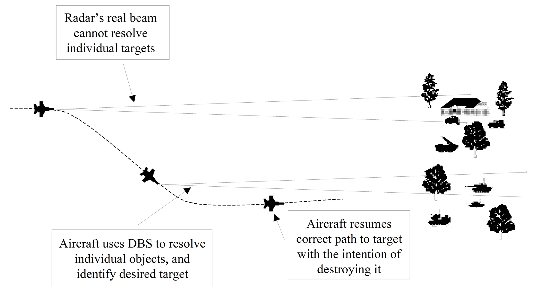
This is an extreme application of forward steering, and is used in strike attack aircraft rather in reconnaissance. Figure 19 illustrates the technique. The aircraft flies in toward its target using a forward-looking real beam. When it has obtained a target in poor resolution, it then changes heading and flies with the target 10º or so off the nose, using the steered real beam to illuminate the target. SAR processing now sharpens up the resolution, and the target is identified. The aircraft then turns back onto its original heading, and attacks the target, confident that it is the correct one.

DBS uses Doppler processing, and also uses a fixed integration time. Thus the bandwidth of the filter, and hence the synthetic beamwidth, is constant. Thus the cross-range resolution degrades with range in the same way that it does in the real beam. However, the synthetic beam has a much narrower beamwidth, hence the name Doppler Beam Sharpening.

Spotlight mode

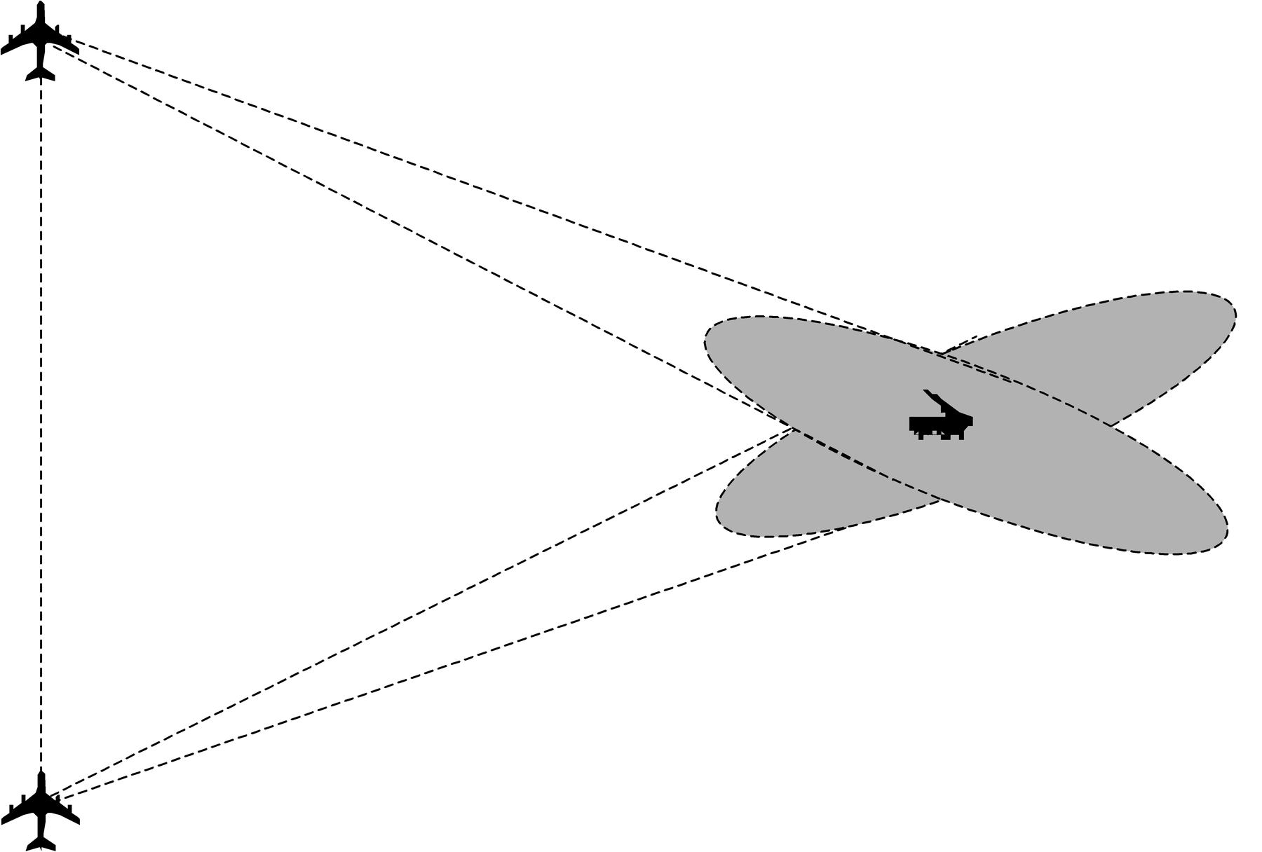
By steering the real beam, it is possible to illuminate a designated patch of ground for much longer than normal. This allows the synthesis of a much longer array, which in turn allows a better cross-range resolution than is possible with a conventional side-looking SAR. Figure 20 illustrates the technique.

Using the frequency history approach, the longer dwell time of the real beam allows the synthesis of a narrower Doppler filter, allowing improved cross-range resolution.

Inverse SAR

In all the discussion so far, it has been the radar platform that has been in motion, and the synthesis of the array has been based on this. Doppler processing also relies on platform motion to produce the required Doppler frequencies. However, it has been mentioned that target motion affects the image detrimentally by displacing or blurring the image. There are operational situations where target motion tends to be present, and this makes the SAR process somewhat inappropriate. (An obvious example is that of a ship, which is subject to a rolling motion in any kind of sea state. This is illustrated in Figure 21.)

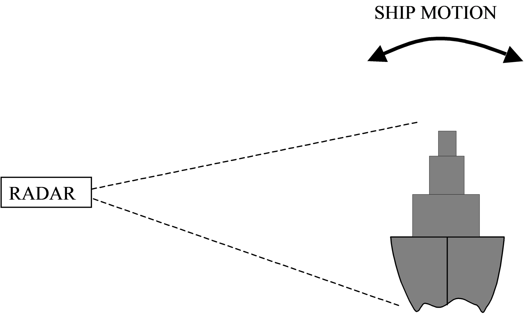
In this situation, it is possible in principle to use the target motion to generate the necessary Doppler frequencies. Imaging using this principle is known as ISAR imaging. The idea is illustrated in Figure 22.

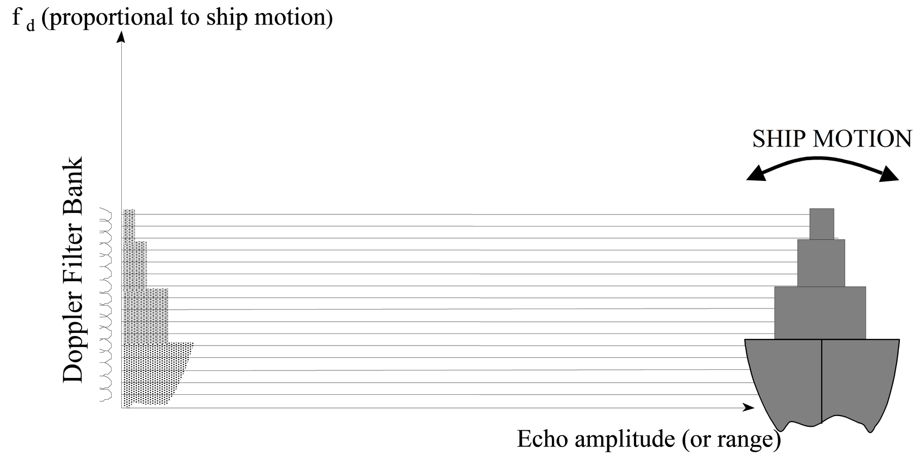
A ship is rolling towards or away from a radar that is illuminating it from the side. Since the top of the ship is moving faster than the hull, it will give a greater Doppler shift to the returning echo. Indeed, the entire vertical structure of the ship will be spread out in Doppler during the roll. One can then resolve vertical detail by using Doppler processing on the returning echo. In its simplest form, the radar plots returning signal strength against Doppler as shown in Figure 22. The vertical profile is then in terms of RCS. With more sophistication, (and very good range resolution), range could be used instead, and then the vertical profile is in terms of the shape of the hull. Horizontal detail may still be obtained by conventional SAR, or the yawing motion of the ship may be used in ISAR. Thus 2-D imaging is possible. In practice, ISAR is successful as a method only when the motion of the target is known reasonably well, and the example of the ship given here is such a situation. However, since precise target motion is not known, the same performance cannot be expected from ISAR on a ship as SAR on a stationary target. Nevertheless, it remains a most promising approach against naval targets.

References

Author

Roger Picton joined Cranfield University in 1987 as a lecturer within the Faculty of Defence Technology and Management. (This Faculty is situated at the Royal Military College of Science, Shrivenham, and provides academic support for the military training that takes place there.) He is currently Head of Radar Systems Group within the Department of Aerospace, Power and Sensors, where he is responsible for the teaching and research in Radar Systems and Radar EW Systems that is carried out there. Prior to joining the Cranfield staff, he spent 16 years in the Royal Air Force carrying various tasks involving the education and training of RAF personnel in the area of Electronic Engineering.

References

[1] G. Stimson, Introduction to Airborne Radar, IEE Press, 1998.
[2] M. Skolnik, Introduction to Radar Systems, McGraw Hill, 1986.
[3] M. Richardson et al, Surveillance and Target Acquisition Systems, Brassey’s, 1997.
[4] J. Curlander and R. McDonough, Synthetic Aperture Radar, John Wiley & Sons, 1991.
[5] G. Galati (Ed), Advanced Radar Techniques and Systems, Peter Peregrinus, 1994.