Performance Of Maximum Likelihood Estimator For Fitting Lanchester Equations On Kursk Battle Data

Introduction

Lanchester [9] based models of warfare provide information that assists decision makers in planning, organization, development and implementation of operational plans. Lanchester equations are widely used for calculating attrition rates in combat modelling. Before 1995, it was believed that the concept of ‘Combat Modelling’ using differential equations was first introduced by Lanchester in 1915 but later Helmbold and Rehm [8] found that similar types of differential equations were already discovered by the Russian author, M. Osipov [12], whose work firstly appeared in the Russian journal Voenniy Sbornik. Helmbold and Rehm [8] had then translated the original work of M. Osipov [12] into English because they believed that Osipov's work was important historically and he should be credited for his contribution. Regardless of credits for prior discovery, Lanchester’s equations form the basis of combat modelling all over the world. The general form of the model to be estimated is:

$${\displaystyle \stackrel{\dot{R}\left(t\right)=\text{bB}\left(t{)}^{p}R\right(t{)}^q}{\dot{B}\left(t\right)=\text{a}\text{R}\left(t{)}^{p}B\right(t{)}^q\left(1\right)}}$$$$$$

where B and R are the strengths of blue and red forces at time t, $${\displaystyle \dot{B}}$$and $${\displaystyle \dot{R}}$$are blue and red forces killed at time t, a and b are daily attrition parameters (weapons loss per day), p is the exponent parameter of the attacking force, and q is the exponent parameter of the defending force.

Equations (1) and (2) involves four unknown parameters (a, b, p and q). Two versions of Lanchester’s equations are of utmost importance. In Lanchester linear law, p=q=1—that is, force ratios remain equal if aR(0)=bR(0). Lanchester’s linear law is interpreted as a model that results from a series of one-on-one duels between homogeneous forces and describes combat under ‘ancient conditions’. The equation is also considered to be a good model for area fire weapons, such as artillery. In Lanchester’s square law, p=1 and q=1—that is, force ratios remain equal if aR(0)²=bR(0)², can be applied to modern warfare in which both sides are able to aim their fire or concentrate forces.

Apart from these two forms, several authors have fitted a number of Lanchester models with different values of p and q to the historical battle data of World War II such as Ardennes Campaign (between Germany and United States), Kursk Campaign (between Soviet and Germany), Iwo-Jima campaign (between United states and Japan). For example, Willard [18] has tested the ability of the Lanchester model for analyzing the historical battle data for the years 1618–1905. He applied the linear regression to the logarithmically transformed Lanchester equations for estimating parameters. Weiss [17] modified Lanchester’s original work for aimed fire (armour battle). Engel’s [5] conducted his study using Iwo-Jima campaign of World War II to validate Lanchester’s square law equation. His dataset consisted of the daily force strengths of American forces and starting and ending force strengths for Japanese forces. Engel [5] concluded that the square law could reasonably account daily US attrition and total Japanese attrition.

Bracken [1] formulated four different models which are the variations of the basic Lanchester equations (1) and (2). Using a constrained grid search, he estimated the parameters (a, b, p, q) for the first 10 days of the Ardennes campaign data with and without an additional defensive parameter for combat forces and total forces. He concluded that the Lanchester linear model best fits the Ardennes campaign data in terms of minimizing the sum of squared residuals (SSR).

Fricker [6] followed up Bracken’s study of the Ardennes campaign of World War II by applying linear regression on the logarithmically transformed Lanchester equations to determine the parameters that provided the best fit when compared to the actual data. He also included air sortie data and employed an algorithm that reconfigured daily force levels to include all reinforcements at the beginning of the campaign. In contrast to the results found by Bracken, Fricker concluded that neither the Lanchester linear nor Lanchester square laws fitted the data. He concluded that force losses depends more on own forces than on the opponent forces. Also, fitting the attrition parameters by linear regression improves the fit of the models as measured by the sum of squared residuals.

Clemens [2] fitted Lanchester equations (1) and (2) to the Battle of Kursk. He estimated the parameters using two different techniques (i) Linear regression on logarithmically transformed equations (ii) a non linear fit to the original equations using a numerical Newton-Raphson algorithm. He concluded that neither of the basic Lanchester laws resulted in a good fit.

Hartley and Helmbold [7] tested Lanchester’s square law using one-sided data from the Inchon-Seoul Campaign. They concluded that data does not fit a constant coefficient Lanchester square law and that a better fit was found if the data is divided into a set of three separate battles. They also concluded that Lanchester’s square law is not a proven attrition algorithm for warfare.

Wiper, Pettit and Young [19] used Bayesian computational techniques to fit the Ardennes Campaign data. They compared their results with the results of the Bracken and Fricker and results were found to be different. They concluded that logarithmic and linear-logarithmic forms fits more appropriately as compared to the linear form found by Bracken. They also concluded that the Bayesian approach is more appropriate to make inferences for battles in progress as it uses the prior information from experts or previous battles. They have applied the Gibbs sampling approach along with Monte Carlo simulation for deriving the distribution patterns of the parameters involved.

Turkes [16] performed a comprehensive analysis by analyzing previous methodologies using different techniques for locating the best fitting parameters and exploring the impact of different weighting schemes to form homogeneous force levels. He employed 39 different models using linear and robust regression. He also applied four separate weight combinations to determine his model’s sensitivity to weighting criteria. He found that none of the basic Lanchester models fit the data correctly and raises the question of utility of the basic Lanchester model for combat modelling.

Lucas and Turkes [10] also tested how Lanchester models fit daily detailed data on the Battles of Kursk and Ardennes. They concluded that none of the basic laws (that is, square, linear or logarithmic) fit the data well. They also suggested finding some new ways to model the attrition as all the previous methods failed to provide a good-fitting Lanchester model.

Reviewing this literature, we found that most of the studies were based on least-square estimation (LSE) approach for fitting the historical battle data. Although this is one of the most commonly used techniques for parameter estimation, there are other approaches such as maximum likelihood estimation (MLE), which have not been explored particularly for fitting historical battle data and finding the parameters involving Lanchester equations. The LSE approaches are useful for obtaining descriptive measures from the data whereas MLE provides the basis for testing hypothesis and constructing confidence intervals. The MLE based estimator possesses many optimal statistical properties such as sufficiency (complete information about the parameter of interest); consistency (sample estimate tends to true parameter value for sufficiently large samples); and efficiency (lowest-possible variance of parameter estimates).

This paper evaluates the performance of the MLE approach, in comparison with other previous approaches such as Bracken [1], Fricker [6], Clemens [2], Wiper et al. [19], Turkes [16], and Lucas and Turkes [10]. All the methodologies applied previously used the LSE technique for fitting the Lanchester equations to the historical battle data. The MLE method [14–15] has not been explored particularly for fitting the historical battle data to date. Also only one measure—sum-of-squared-residuals (SSR)—has been explored for measuring the goodness-of-fit (GOF). The main objective of this study is to assess the performance of the MLE approach for fitting Lanchester equations to the Battle of Kursk. Various measures of GOF [4]—viz. Kolmogorov-Smirnov, Chi-square and R²—have been computed for comparing the fits and to test how well the model fits the observed data. The performance of MLE technique is validated by applying the various GOF measures considering the artillery strength and casualties of Soviet and German sides from the Kursk battle data of World War-II. Section 2 presents the mathematical derivations for estimating the parameters using MLE. Section 3 describes the artillery data of Battle of Kursk and discusses the methodology for implementing the proposed as well as other approaches. Also, this section contains a performance appraisal of the MLE using various GOF measures. Section 4 analyzes the results after observing various tables and figures and discusses how well the MLE fits the data. Section 5 summarizes the important aspects of the paper.

MAXIMUM LIKELIHOOD ESTIMATION

The MLE estimation [14–15] begins with writing a mathematical expression known as the likelihood function of the sample data. The likelihood of a set of data is the probability of obtaining that particular set of data, given the chosen probability distribution. This expression contains the unknown parameters. The values of these parameters that maximize the sample likelihood are known as the maximum likelihood estimates or MLE. The principle of MLE states that the desired probability distribution is the one that makes the observed data ‘most likely’.

Let (B_n,R_n) represents the force strengths of blue and red forces of a battle for the n^th day and N is the duration of the battle. Let the blue and red casualties $${\displaystyle \dot{B}}$$ and $${\displaystyle \dot{R}}$$ in a combat are two random variables whose densities are $${\displaystyle f_{\dot{B}}\left(S\right|B,R,a,p,q)=f(S|B,R,a,p,q)}$$and $${\displaystyle f_{\dot{R}}\left(S\right|R,B,b,p,q)=f(S|R,B,b,p,q)}$$ respectively, where the forms of the densities are assumed to be known except that these contain unknown parameters$${\displaystyle a,b,p,q}$$. Further it is assumed that the casualties $${\displaystyle {\stackrel{\text{.}}{(B}}_1,{\stackrel{\text{.}}{B}}_2,\text{.}\text{.}\text{.},{\stackrel{\text{.}}{B}}_n)}$$ and $${\displaystyle ({\stackrel{\text{.}}{R}}_1,{\stackrel{\text{.}}{R}}_2,\text{.}\text{.}\text{.},{\stackrel{\text{.}}{R}}_n)}$$of a random sample $${\displaystyle (B_n,R_n)}$$ from $${\displaystyle f\left(S\right|B,R,a,p,q)}$$ or $${\displaystyle f\left(S\right|R,B,b,p,q)}$$ can be observed. On the basis of the observed sample values $${\displaystyle {\stackrel{\text{.}}{(B}}_1,{\stackrel{\text{.}}{B}}_2,\text{.}\text{.}\text{.},{\stackrel{\text{.}}{B}}_n,{\stackrel{\text{.}}{R}}_1,{\stackrel{\text{.}}{R}}_2,\text{.}\text{.}\text{.},{\stackrel{\text{.}}{R}}_n)}$$ it is desired to estimate the values of the unknown parameters a, b, p and q. We further assume that the times between casualties are exponentially distributed, then the probability density function or pdf of inter-casualty times for the Red (R) and Blue (B) sides associated to the equations (1) and (2) can be represented as in the equations (3) and (4) :

$${\displaystyle f_{\stackrel{\text{.}}{B}}\left(S\right|B,R,a,p,q)=\begin{array}{c}\left\{a{R}^p{B}^q{e}^{-\left(a{R}^p{B}^q\right)s},R,B>0,-\infty \le a,p,q\le \infty ,0\le s\le \infty \right|\end{array}\\ }$$ (3)

$${\displaystyle f_{\stackrel{\text{.}}{R}}\left(S\right|R,B,b,p,q)=\begin{array}{c}\left\{b{B}^p{R}^q{e}^{-\left(b{B}^p{R}^q\right)s},R,B>0,-\infty \le b,p,q\le \infty ,0\le s\le \infty \right|\end{array}\\ }$$ (4)

The likelihood function of n pairs of random variables $${\displaystyle {\stackrel{\text{.}}{(B}}_1,{\stackrel{\text{.}}{B}}_2,\text{.}\text{.}\text{.},{\stackrel{\text{.}}{B}}_n,{\stackrel{\text{.}}{R}}_1,{\stackrel{\text{.}}{R}}_2,\text{.}\text{.}\text{.},{\stackrel{\text{.}}{R}}_n)}$$ is defined as the joint density of the n pairs of random variables, say $${\displaystyle f_{\dot{B},\dot{R}}(R_n,B_n|a,b,p,q)}$$ which is considered to be a function of a, b, p, q. In particular, if $${\displaystyle {\stackrel{\text{.}}{(B}}_1,{\stackrel{\text{.}}{B}}_2,\text{.}\text{.}\text{.},{\stackrel{\text{.}}{B}}_n,{\stackrel{\text{.}}{R}}_1,{\stackrel{\text{.}}{R}}_2,\text{.}\text{.}\text{.},{\stackrel{\text{.}}{R}}_n)}$$ are identically and independently distributed (i.i.d.) random sample from the density$${\displaystyle f(R,B|a,b,p,q)}$$, then the likelihood function is

$${\displaystyle f\left(s\right|B_1,a,p,q\left)f\right(s|R_1,b,p,q),f\left(s\right|B_2,a,p,q\left)f\right(s|R_2,b,p,q),\text{.}\text{.}\text{.},f\left(s\right|B_n,a,p,q\left)f\right(s|R_n,b,p,q)\text{.}}$$

The joint pdf is given by the equation:

$${\displaystyle f_{{\dot{B}}_1,{\dot{R}}_1,{\dot{B}}_2,{\dot{R}}_2\dots {\dot{B}}_n,{\dot{R}}_n}\left(S\right|R,B,a,b,p,q)=\left\{{\text{aR}}_n^p{B}_n^q+{\text{bB}}_n^p{R}_n^q\right\}{e}^{-({\text{aR}}_n^p{B}_n^q+{\text{bB}}_n^p{R}_n^q)s},}$$ (5)

0$${\displaystyle \left({\dot{B}}_1,{\dot{R}}_1\right),\left({\dot{B}}_2,{\dot{R}}_2\right),\dots ,\left({\dot{B}}_n,{\dot{R}}_n\right)<\infty }$$

To construct the likelihood function from the available dataset, it is generally observed that casualty figures are generally available at daily interval. Let $${\displaystyle L(a,b,p,q)}$$be the likelihood function for the random variables $${\displaystyle {\stackrel{\text{.}}{(B}}_1,{\stackrel{\text{.}}{B}}_2,\text{.}\text{.}\text{.},{\stackrel{\text{.}}{B}}_n,{\stackrel{\text{.}}{R}}_1,{\stackrel{\text{.}}{R}}_2,\text{.}\text{.}\text{.},{\stackrel{\text{.}}{R}}_n)}$$. If $${\displaystyle \widehat{a},\widehat{b},\widehat{p},\widehat{q}}$$is the value of $${\displaystyle a,b,p,q}$$ which maximizes$${\displaystyle L(a,b,p,q)}$$, then $${\displaystyle \widehat{a},\widehat{b},\widehat{p},\widehat{q}}$$ are the maximum-likelihood estimates of $${\displaystyle a,b,p,q}$$.

Thus, the likelihood function is given by the equation:

$${\displaystyle L(s,a,b,p,q)={\prod }_{n=1}^N({\text{aR}}_n^p{B}_n^q{)}^{{\dot{B}}_n}\times ({\text{bB}}_n^p{R}_n^q{)}^{{\dot{R}}_n}\text{e}\text{x}\text{p}\left\{-\left({\text{aR}}_n^p{B}_n^q+{\text{bB}}_n^p{R}_n^q\right)s\right\}\\ }$$ (6)

Now, instead of maximizing the likelihood function we maximize its logarithmic form since both the maximum values occur at the same point and the logarithmic form is readily computable.

Thus, on taking the log of equation (6), we have the following equation:

$${\displaystyle \text{ln}L={\sum }_{n=1}^N{\dot{B}}_n\text{ln}\left({\text{aR}}_{n^p}{B}_{n^q}\right)+{\sum }_{n=1}^N{\dot{R}}_n\text{ln}\left({\text{bB}}_{n^p}{R}_{n^q}\right)-{\sum }_{n=1}^N\left({\text{aR}}_n^p{B}_n^q+{\text{bB}}_n^p{R}_n^q\right)s}$$ (7)

Differentiating the log-likelihood function (7) partially with respect to a and b and equating it to zero, we have:

$${\displaystyle \frac{d\text{ln}L}{\text{da}}=\frac{d}{\text{da}}{\sum }_{n=1}^N{\dot{B}}_n\left(\text{log}a+p\text{log}{R}_n+q\text{log}{B}_n\right)-{\sum }_{n=1}^N{R}_n^p{B}_n^{q}s=0}$$

and:

$${\displaystyle \frac{d\text{ln}L}{\text{db}}=\frac{d}{\text{db}}{\sum }_{n=1}^N{\dot{R}}_n\left(\text{log}b+p\text{log}{B}_n+q\text{log}{R}_n\right)-{\sum }_{n=1}^N{B}_n^p{R}_n^{q}s=0}$$

This gives:

$${\displaystyle {\sum }_{n=1}^N\frac{{\dot{B}}_n}{a}-{\sum }_{n=1}^N{R}_n^p{B}_n^{q}s=0}$$ and

$${\displaystyle {\sum }_{n=1}^N\frac{{\dot{R}}_n}{b}-{\sum }_{n=1}^N{B}_n^p{R}_n^{q}s=0}$$

Thus, the maximum likelihood estimates are given by the equations:

$${\displaystyle \widehat{a}=\frac{{\sum }_{n=1}^N{\dot{B}}_n}{{\sum }_{n=1}^N{R}_n^p{B}_n^{q}s}}$$ (8)

$${\displaystyle \widehat{b}=\frac{{\sum }_{n=1}^N{\dot{R}}_n}{{\sum }_{n=1}^N{B}_n^p{R}_n^{q}s}}$$ (9)

This implies:

$${\displaystyle {\sum }_{n=1}^N{R}_n^p{B}_n^{q}s=\frac{{\sum }_{n=1}^N{\dot{B}}_n}{\widehat{a}}}$$

$${\displaystyle {\sum }_{n=1}^N{B}_n^p{R}_n^{q}s=\frac{{\sum }_{n=1}^N{\dot{R}}_n}{\widehat{b}}}$$

Taking the logarithm of the above two equations, we have:

$${\displaystyle \text{ln}\left({\sum }_{n=1}^N{R}_n^p{B}_n^q\right)s=\text{ln}\left({\sum }_{n=1}^N\stackrel{\text{.}}{B_n}\right)-\text{ln {}\widehat{a}}$$ (10)

$${\displaystyle \text{ln}\left({\sum }_{n=1}^N{B}_n^p{R}_n^q\right)s=\text{ln}\left({\sum }_{n=1}^N\stackrel{\text{.}}{R_n}\right)-\text{ln {}\widehat{b}}$$ (11)

Unfortunately no explicit solution for $${\displaystyle \widehat{p},\widehat{q}}$$ is possible. We propose to use the generalized reduced gradient method [13] to solve equations (8) and (9) simultaneously to obtain the desired MLEs of a and b.

DATA USED AND METHODOLOGY

The largest tank battle in World War II, popularly known as the Battle of Kursk, was fought between Soviet and Germany in July 1943 around the city of Kursk. A detailed database has been developed by the Dupuy Institute and was reformatted into a computerized database known as the Kursk Data Base (KDB) in 1998. KDB is documented in the KOSAVE (Kursk Operation Simulation and Validation Exercise) [3]. It mainly consists of units and combat posture status, personnel status and casualties, Army weapons status and losses, ammunition status, aircraft sortie status and geographic unit positions and progress. The KDB contains daily weapons on hand and losses for the four categories—namely, manpower, tanks, APC and artillery for the Soviets and Germans for each of the 15 days of battle. In the present study, we have considered only the artillery data for validating the performance of the MLE for fitting battle data. Table 1 shows the artillery weapons on hand and losses during the 15 days battle. Figure 1 shows a comparison between the Soviet and German losses during the 15 days battle. From this figure, we observe that Soviets had high casualties on the third day of the battle. Also, the Germans had lost 144 artillery guns in total as compared to 127 of the Soviet Artillery guns. On the 8^th and 15^th days of the battle, the Germans had sustained more casualties than Soviets. Therefore, it is quite obvious that there is a non-linear relationship in the distribution pattern of the two forces. Table 1 shows Total Artillery Weapon strength and Losses.

This paper fits the generalized form of Lanchester equations to the Battle of Kursk data using the method of MLE and compares the performance of MLE with the techniques studied earlier such as the sum of squared residuals (SSR), linear regression and Newton-Raphson iteration. Different authors applied different methodologies for fitting Lanchester equations to the different battle data. The methodologies of Bracken, Fricker, and Clemens are applied to the artillery data of Battle of Kursk and results are shown in Table 2.

For implementing Bracken’s approach, the technique of Sum of Squared Residuals (SSR) was applied on the artillery data given in Table 1 by locating the best fitting parameters which minimize the SSR between the actual and estimated attrition. Using 15 days data of the Battle of Kursk, where the first 8 days the Germans attack and the last 7 days the Soviets attack, we desired to minimize:

$$$$$${\displaystyle \text{S}\text{S}\text{R}={\sum }_{n=1}^8{\left({\dot{B}}_n-{\text{aR}}_n^p{B}_n^q\right)}^2+{\sum }_{n=1}^8\left({\dot{R}}_n-{\text{bB}}_n^p{R}_n^q\right)+{\sum }_{n=9}^{\text{15}}{\left({\dot{B}}_n-{\text{aR}}_n^p{B}_n^q\right)}^2+{\sum }_{n=9}^{\text{15}}{\left({\dot{R}}_n-{\text{bB}}_n^p{R}_n^q\right)}^2}$$ (14)

Where n denotes the index for 15 days of the battle. The best model parameters are located by searching over a grid in the {a, b, p, q} space for the minimum sum of square residuals (SSR). The search considered:

$${\displaystyle 0\le \text{p,q}\le 2\text{.}\text{0}}$$and $${\displaystyle 4\times {\text{10}}^9\le \text{a,b}\le 1\text{.}2\times {\text{10}}^{-8}\text{.}}$$

For the application of Fricker’s methodology, we transformed the basic Lanchester equations (1) and (2) to a logarithmic form and applied linear regression on the logarithmically transformed equations. After the logarithmic transformations, the basic Lanchester equations given in (1) and (2) become:

$${\displaystyle \text{l}\text{n}\left(\dot{B}\right)=\text{l}\text{n}\left(a\right)+p\text{l}\text{n}\left(R\right)+q\text{l}\text{n}\left(B\right)\text{l}\text{n}\left(\dot{R}\right)=\text{l}\text{n}\left(b\right)+p\text{l}\text{n}\left(B\right)+q\text{l}\text{n}\left(R\right)}$$ (15)

Linear regression was applied on equation (15) using the artillery data given in Table 1 and best fitting parameters were obtained.

Clemens study was similar to Fricker in one of his two approaches. He also applied linear regression on logarithmically transformed equations and a non-linear fit to the original equations (1) and (2) was made using a numerical Newton-Raphson algorithm.

Our measure of fit is the MLE technique. The objective is to find the parameters that maximize the log-likelihood or in other words provide the best fit. Given the values in Table 1, we investigated what values of the parameters (a, b, p, q) best fit the data.

We used the Generalized Reduced Gradient (GRG) method for maximizing the likelihood function and thence to obtain the MLE of the parameter. The GRG algorithm is available with the Microsoft Office Excel (2007) Solver [13]. The GRG solver uses iterative numerical method. The derivatives (and Gradients) play a crucial role in GRG. The basic idea of using GRG algorithm is to quickly find optimal parameters that maximize the log-likelihood. Although we derived the estimates for a and b using the MLE approach in equations (8) and (9), they are not applied directly. Log likelihood is calculated using equation (7) by initializing the parameters on the first day of the battle as a(0)=1, b(0)=1, p(0)=1 and q(0)=1. We break the battle into several phases, each of which is assumed to be relatively homogeneous. Also, the extremely low casualty levels on the first day represent large outliers; thus, including the data of the first day affects the outcome to a great extent. Thus, the first day was dropped in fitting the data to the models. This approach is also justified by the historical account of the battle of Kursk, because the fight did not begin until July 5, the second day of the battle.

Thus, dropping the data for the first day and dividing the remaining 14 days data into five phases, Log-likelihood is calculated using equation (7) and is maximized separately for each of the five phases. Let d denote the days, then the division is made as (d₂-d₃), (d₄-d₆), (d₇-d₈), (d₉-d₁₁), and (d₁₂-d₁₅). Fitting the model over multiple phases results in a better overall fit because there are additional parameters to explain the variation in casualties.

For the purpose of comparing models, R² value is calculated along with the SSR. The R² value is calculated as:

$${\displaystyle R^2=1-\frac{\text{SSR}}{\text{SST}}=1-\frac{{\sum }_{n=1}^{\text{15}}{\left({\dot{B}}_n-{\dot{\widehat{B}}}_n\right)}^2+{\sum }_{n=1}^{\text{15}}{\left({\dot{R}}_n-{\dot{\widehat{R}}}_n\right)}^2}{{\sum }_{n=1}^{\text{15}}{\left({\dot{B}}_n-\overline{B}\right)}^2+{\sum }_{n=1}^{\text{15}}{\left({\dot{R}}_n-\overline{R}\right)}^2}}$$

where $${\displaystyle \overline{R}}$$ and $${\displaystyle \overline{B}}$$ denote the mean value of the daily force losses for the Germans and Soviets respectively and $${\displaystyle {\dot{\widehat{B}}}_n}$$ and $${\displaystyle {\dot{\widehat{R}}}_n}$$ are the estimated values of the Soviet and German casualties respectively. Larger R² values indicates better fit. Also, goodness-of-fit measures namely, Kolmogorov-Smirnov statistic [4] and Chi-square ($${\displaystyle {\chi }^2}$$) [4] have been calculated for the accuracy assessment of the MLE to that of the conventional approaches. Kolmogorov-Smirnov statistic is a measure of goodness-of-fit, that is, the statistic tells us how well the model fits the observed data. The Kolmogorov-Smirnov (KS) statistic is based on the largest vertical difference between the theoretical and empirical (data) cumulative distribution function.

$${\displaystyle \text{KS}=\underset{1\le n^{}\le \text{30}}{\text{max}}\left[F\left({\dot{\widehat{e}}}_{n^{}}\right)-\frac{n^{}-1}{\text{30}},\frac{n^{}}{\text{30}}-F\left({\dot{\widehat{e}}}_{n^{}}\right)\right]}$$

where $${\displaystyle F\left({\dot{\widehat{e}}}_{n^{}}\right)}$$ is the cumulative distribution function of the estimated error between the observed losses and the estimated losses for both sides. Chi-Square ($${\displaystyle {\chi }^2}$$) is another measure of Goodness-of-fit. Chi-Square is given as:

$${\displaystyle {\chi }^2={\sum }_{n=1}^{\text{15}}\frac{{\left({\dot{B}}_n-{\dot{\widehat{B}}}_n\right)}^2}{{\dot{\widehat{B}}}_n}+{\sum }_{n=1}^{\text{15}}\frac{{\left({\dot{R}}_n-{\dot{\widehat{R}}}_n\right)}^2}{{\dot{\widehat{R}}}_n}}$$

where $${\displaystyle {\dot{\widehat{B}}}_n}$$ and $${\displaystyle {\dot{\widehat{R}}}_n}$$ are the estimated values of the Soviet and German casualties respectively.

Results and Discussions

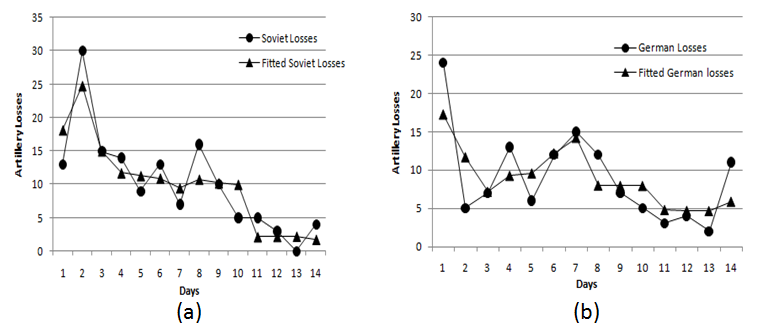
Figure 3.3D and contour plots of least square and likelihood based estimation obtained after analysing the artillery data of the Soviet and German sides from the Kursk battle. (a) SSR and (b) log-likelihood (c) Contour plot of SSR (d) contour plot of log-likelihood values.Figure 3.3D and contour plots of least square and likelihood based estimation obtained after analysing the artillery data of the Soviet and German sides from the Kursk battle. (a) SSR and (b) log-likelihood (c) Contour plot of SSR (d) contour plot of log-likelihood values.

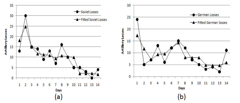
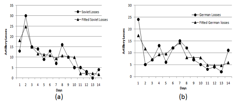
Figures 2 (a) and 2 (b) show the fitted losses plotted versus real losses for the Soviet and German Artillery data respectively, by dropping the data for the first day and dividing the remaining data into 5 phases. From the figures, it is apparent that fitting the models with division into several phases fits quite well. Table 2 shows the results of Bracken, Fricker, Clemens and MLE applied on the artillery data. This table shows the KS statistic for MLE (with division) is 0.10534, which is less than any other estimation methods implying that the method of MLE fits better as compared to the other methods. Also, R² is a measure of goodness of fit. Larger values of R² implies a good fit to the data. The R² value of MLE (with division) is 0.7279, highest among the other estimation methods. For comparing the efficiency of the different approaches, the root mean square error (RMSE) criteria is used. The RMSE of MLE with 5 divisions is 6.02 which is found to be the minimum. The RMSE of Fricker’s model is 12421.1 which is found to be the maximum. Therefore, efficiency (E) is measured with respect to the RMSE of the MLE. Thus, the E for MLE is maximum (that is, equal to 1) and E of Frickers’s model is minimum (that is, equal to 0.000485). If the comparison is made among Bracken's, Fricker's and Clemens approaches, we can say that the Bracken approach is better. However, in all the cases the MLE outperforms other approaches. Based on all the GOF measures, it can be concluded that MLE provides better fits.

Figure 3(a) shows the 3D plot of SSR values found for the battle of Kursk artillery data where p and q values are varied between 0 and 10, a and b values depend on p and q and are determined by equations (8) and (9). The surface area and contour plots are generated using the MATLAB software [11]. Figure 3(c) shows area using the contour plot of the minimum SSR as a function of p and q. A contour plot displays the contours of equally fitting p and q values in terms of SSR. From this figure we can see that the minimum SSR zone is represented by the contour of 1,300. Using a grid search in this zone the best, or optimal, fit is obtained at p=1.4 and q=3 with an SSR value of 1,300. The a and b values corresponding to the optimal fit are 1.8465E-12 and 6.8569E-13 respectively. This indicates that, individually, the Germans were more effective as compared to the Soviets since a and b are the attrition rates (weapons loss per day) of Soviets and Germans respectively (a>b). These estimates are obtained using exhaustive search algorithm implemented in the MATLAB software. Also, Figure 3(b) shows the 3D plot of Log-likelihood values for the Artillery data of the Kursk Battle. The parameters are estimated through maximizing the log-likelihood function using (7). Figure 3(d) shows the contour plot of the maximized log-likelihood equation (7) as a function of p and q. This contour plot displays the contours of equally fitting p and q values in terms of Likelihood function. From this figure, it can be seen that the maximum likelihood zone is represented by the contour of 330. Using a grid search in this zone, the best fit is obtained at p=2.2 and q=4.4 with a log-likelihood of 332.26. This signifies that force losses depends on both the forces but more on its own forces (q>p). The a and b values corresponding to the optimal fit are 7.5248E-19 and 1.7150E-19 respectively. This implies that, individually, the Germans were more effective than the Soviets since a and b are the attrition rates (weapons loss per day) of Soviets and Germans respectively (a>b). Similar to the least square estimation, these estimates are obtained using exhaustive search algorithm implemented in the MATLAB software.

Conclusions

Lanchester equations and their extensions are widely used in the field of research and decision making process. Different authors applied different techniques for fitting Lanchester models to the battle of Kursk and came up with different results. For the first time, we applied the MLE technique for fitting Lanchester models to the Battle of Kursk and found different estimates of a, b, p and q. The failure to find a good-fitting model by the previous approaches motivated us to explore MLE. We do not restrict ourselves to the basic Lanchester laws (linear, square or logarithmic). The MLE estimates obtained possess the optimum properties of sufficiency, consistency and efficiency. The MLE estimates are sufficient in the sense that they contain all the relevant information about the parameters and are always consistent. Further, the efficiency of MLE is highest when compared to the other estimation methods as can be seen from the results. Thus, it can be concluded that the approach of MLE is statistically more accurate and provides much better fits than with the previous approaches. The artillery data of the Battle of Kursk was used for comparing the approaches studied previously with the proposed approach of MLE because we wanted to explore the rationale of MLE approach for fitting Lanchester models to the battle data. The MLE approach can be applied to tank, APC and manpower data of the Kursk campaign of World War II.

References

Author

Manvi Sahni is a research fellow at the Institute for Systems Studies and Analyses, Delhi, India. She has an MSc in statistics from the Faculty of Mathematical Sciences, University of Delhi, Delhi, India. E-mail : ms.manvi91@gmail.com.

Sumanta Kumar Das is a scientist at the Institute for Systems Studies and Analyses, Delhi, India. His research interests include machine intelligence, pattern recognition, and remote sensing. Das has a PhD in agricultural statistics from the Indian Agricultural Research Institute (IARI), New Delhi, India. E-mail: skdas@issa.drdo.in.

References

J. Bracken, “Lanchester Models of the Ardennes Campaign”, Naval Research Logistics, Vol. 42, 1995, pp. 559–577.
S. Clemens, The Application of Lanchester Models to the Battle of Kursk, unpublished manuscript, Yale University, New Haven, CT, 5 May 1997.
Centre for Army Analysis, Kursk Operation Simulation and Validation Exercise—Phase II (KOSAVE II), The US Army’s Centre for Strategy and Force Evaluation Study Report, CAA-SR-98-7, Fort Belvoir, VA, September 1998.
R. D’Agostino and M.A. Stephens, Goodness-of-fit Technique, 68, 1986.
J. Engel, “Verification of Lanchester’s Law”, Operational Research, Vol. 2, 1954, pp. 163–171.
R. Fricker, “Attrition Models of the Ardennes Campaign”, Naval Research Logistics, Vol. 45, 1998, pp. 1–22.
D. Hartley and R. Helmbold, “Validating Lanchester’s Square Law and Other Attrition Models”, Naval Research Logistics, Vol. 42, 1995, pp. 609–633.
R. Helmbold and A. Rehm, “The Influence of the Numerical Strength of Engaged sides on Their Casualties by M. Osipov”, Naval Research Logistics, Vol. 42, 1995, pp. 435–490.
F. Lanchester, Aircraft in Warfare: The Dawn of the Fourth Arm, Constable, London, 1916.
T. Lucas and T. Turkes, “Fitting Lanchester Equations to the Battles of Kursk and Ardennes”, Naval Research Logistics, vol. 51, 2004, pp. 95–116.
MATLAB The Language of Technical Computing, Version 7.0. 4. 365 (R14), 2006.
M. Osipov, “The Influence of the Numerical Strength of Engaged Sides on their Casualties”, Voenniy Sb (Military Coll), 1915, pp. 6–10.
Microsoft Excel Solver User’s Guide for Windows, version 3.0, p. 2.
V. Rohatgi, Statistical Inference, Wiley Series in Probability and Mathematical Statistics, 1984.
J. Taylor, Lanchester Models of Warfare 2, Military Applications Section, Operations Research Society of America, Alexandria, VA, 1983.
T. Turkes, Fitting Lanchester and Other Equations to the Battle of Kursk Data, Master's Thesis, Department of Operations Research, Naval Postgraduate School, Monterey, CA, March 2000.
H. Weiss, “Lanchester-type Models of Warfare”, Proceedings of the First International Conference on Operational Research, 1975, pp. 82–98.
D. Willard, Lanchester as Force in History: An Analysis of Land Battles of the Years 1618-1905, DTIC No. AD297275L, Alexandria, VA, 1962.
M. Wiper, L. Pettit and K. Young, “Bayesian Inference for a Lanchester Type Combat Model”, Naval Research Logistics, Vol. 47, 2000, pp. 541–558.