
Volume 18, Number 1, March 2015
Improving Mission Survivability Of UGV Using Polynomial Non-Linear Regression For Power Prediction
Abstract
Accurate prediction of required energy is essential for efficient deployment of Unmanned Ground Vehicles (UGV). Typical UGV missions do not allow for the replenishment of power resources so mission survivability and overall mission success rate are reliant on accurate power prediction. The live prediction of resources required for a particular mission is therefore beneficial as it could allow for increased mission time and lessen the requirement of over provisioning power resources. Accurate power prediction has particular importance when considering critical missions where failure to complete atomic mission operations may lead to an unsafe situation. This paper presents a new approach to live energy prediction that considers the effects of weather conditions on off-road terrains based upon non-linear polynomial regression for prediction of mission energy consumption using live sensor data. The method is demonstrated and compared to existing methods using a simulation of a typical UGV mission. The mission simulation considers a UGV traversing a variety of terrain types in various weather conditions. The experimental results show a significant improvement in energy prediction compared to existing approaches and demonstrates the success of forward prediction using non-linear terrain/weather/energy consumption models.
Introduction
Unmanned Ground Vehicles (UGV) are becoming more widespread in their deployment due to advances in technology regarding machine intelligence, sensing hardware and perception algorithms [1]. Typical applications include surveillance, transportation, mine clearing and search and rescue. UGV are well suited to applications that are considered dull, dirty or dangerous or for where it is physically impossible for humans to venture, for example planetary exploration [2]. As technology advances further, UGV will be required to participate in increasingly complex missions.
To further stretch the possibilities of UGV missions, much focus on the development of UGV is the research of autonomy and the ability to plan routes and navigate long distances through unstructured environments which consist of differing terrain types which, in turn, are affected by dynamic variables such as influences of weather [1,3,4]. To achieve this, methods such as object avoidance, situational awareness and complex path planning are required. For this to be possible more hardware is required (such as sensors for object recognition, and GPS for navigation assistance) and more processing power is required to control this additional functionality.
This additional functionality puts an extra burden on the already stretched power resources available to UGV. Most small UGV are fitted with power sources with limited reserves such as battery packs and minimal recharging facilities. This power reserve limitation can be a restricting factor to the future abilities of UGV and limit their flexibility to cope with various mission types. An example is limited mission duration, where a UGV operational period is directly affected by remaining power reserves. In military applications (but not limited to) it is typical that mission plans change dynamically during mission time and remaining resources will influence the possibilities available to mission planners and could restrict the likelihood of mission success. In safety critical operations, such as UGV deployed by emergency services, it is of utmost importance that a UGV has enough power reserve to complete a task rather than creation of an unsafe environment through mission abortion due to depleted power.
Accurate prediction of mission power requirements goes some way to address many such situations. In the example of limited mission duration, accurate power prediction may allow operators to increase mission duration by identifying more efficient mission strategies. For dynamic missions, accurate power prediction requirements create strategic mission options as it allows for selection or rejection of opportunities as they may arise. The operator would be able to forecast whether remaining power is adequate for completion of mission opportunities as they arise. For safety critical missions, being able to forecast accurately power reserves allows safe completion of atomic operations, where partial completion would result in an unsafe situation.
Currently, many UGV do not utilise a Power Management System (PMS) that incorporates a capability to perform predictions of future mission power requirements (or no PMS at all) and is considered desirable as opposed to mandatory by Morley [4]. In the absence of mission power prediction, there is a tendency to over-provide regarding energy storage, which impacts on the size and mass of the UGV [4], which will in turn effect and possibly impede transport and deployment methods of a particular UGV, as well as inhibit its manoeuvrability.
At its most rudimentary level, power prediction could be effected offline by utilising prior knowledge of UGV performance regarding propulsion consumption from previously collected data and used to predict the power consumption through a future mission. The accuracy of the prediction could be improved upon dynamically during a live mission by utilising live accurate sensor data that would compensate for any inaccuracies of the prior knowledge or fluctuating dynamic variables (for example, influences of weather). The accuracy of the dynamic prediction would depend on the available sensor data, but with minimal overhead in processing power and by utilising data from standard sensors (GPS, current/voltage sensors) a significant improvement compared to the offline prediction should be affected.
Rolling resistance and its effects on prediction
Depending on the physical size of the UGV and the mission type to be undertaken, a large proportion of energy consumption is due to the propulsion of the UGV [5]. The rate of consumption is dependent on the velocity, the grade (incline) of the terrain being traversed, the rolling resistance coefficient (f) of the terrain and air resistance encountered. Rolling resistance has more impact on consumption when a vehicle is traversing off-road with unforgiving terrain compared to typical road surfaces, which is the likely case for military UGV.
Resource prediction for UGV is similar in context to residual range estimation for electric road vehicles, however the rolling resistance value for road vehicles is much easier to predict due to resistance being similar for most road surfaces compared to off-road terrain types. Prediction is further hampered for off-road vehicles when considering that resistance coefficients for terrain types can change (more dramatically) due to influences of weather (moisture content being the most prevalent), that have a large effect on resistance and hence power consumption.
Rolling resistance when considering vehicles traversing prepared surfaces (concrete, macadam etc) is primarily effected by the deformation of the tyre [6], the additional effect (of most importance) when traversing unprepared terrain (opposed to road surfaces) is the deformation of the terrain surface [7]. Although average values of resistance when considering road vehicles are well documented [7], this is not the case when considering off road vehicles.
The resistance coefficient (f) impacts not only energy consumption but also the maximum permissible velocity of a UGV while traversing a certain terrain, so the accurate prediction of f is equally important when the cost of route traversal is defined by both time and energy. It also may be the case that if a particular terrain type becomes influenced by a certain weather condition then it may be un-navigable by a UGV which further highlights the benefits of accurate rolling resistance prediction.
Related work
Often a UGV is directed to follow a pre-planned route or navigate among predefined waypoints generated by an offline planning algorithm using coarse topographical map data [8]. It is of obvious benefit to characterise the terrain in advance in order to predict both trafficability and vehicle performance over a given route (including power consumption).
The opportunity to have pre-mission information regarding terrain types has improved in recent years with the availability of systems to assess terrain types from aerial imagery [9] and the growth of geographical information systems [10].
From this, a pre-mission prediction can be made regarding consumption accounting for expected rolling resistance values. Unfortunately, it is unlikely that the prior assessment of predicted consumption will be perfectly accurate (at least for a portion of the mission) due to fluctuating resistances (due to weather effects) or not entirely accurate prior information.
Zheng and Reif [10] propose a method for computing energy minimising optimal paths, although variance of f is considered for different terrains, any unexpected variance during a live mission is not considered. Sadrpour [11], proposes a method for online prediction and evaluation using a Bayesian Estimation to take advantage of prior information and online samples of consumption to accurately predict values of f. However, this method only adjusts the prediction for terrain types already traversed (based on live data values) on a predefined route, and assumes that any new resistances for un-traversed terrains are as prior values and also that prior information about terrain types is entirely accurate. It also considers the problem of prediction to be linear in nature, which is not necessarily the case when considering consumption of a UGV that has to contend with steep inclines and varying factors such as excessive “wheel slip”.
Predicting rolling resistance values of yet to be traversed terrain types (based on actual data samples from already traversed terrain types) is considered difficult as influences such as moisture will have varying effects on different terrain types [12]. Considering that net power consumption (considering only longitudinal motion and ignoring aerodynamic force due to the low operating velocities of UGV) for an electrically propelled UGV can be given as [5]:
| (1) |
|---|
where is vehicle weight, the total traction force, the rolling resistance coefficient (equal to ff + fr from Figure 1), the mass, acceleration, is velocity, is the modelling error and where is the effect of incline and the effect of rolling resistance, (see Figure 1).
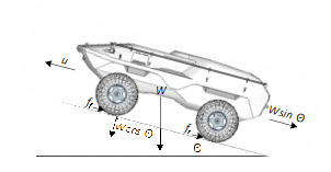
Using typical on-board sensors (for incline, velocity, current and voltage) it would be possible to sample data at a given frequency and conclude a value for rolling resistance. However, the model (1) should only be considered for favourable surfaces typical for road vehicles [13] where resistance is primarily due to deformation of tyres [6,7].
Off-road vehicles rolling resistance values are highly affected by deformation of the terrain surface which has two factors, vertical (terrain deformation due to vehicles weight, i.e. sinking) and horizontal (deformation due to wheel slip) [13]. Further to the issue of prediction of energy requirements, calculation or measurement of resistance coefficient for a particular UGV over varying terrains has not been fully explored [13].
Terrain identification utilising offline methods has received significant attention over the past 40 years, these methods commonly involve human intervention, an example being the “cone penetrometer” (in its simplest form a tool with a conical tip manually pushed into a terrain) whose use to “identify terrain characteristics from the vehicle mobility or terrain trafficability viewpoint remains controversial” [14]. This is opposed to methods of terrain identification using live on-board sensor data which although have been researched [15] is in its infancy. Two primary methods exist, vision based and wheel-terrain interaction analysis. Research to date is for the primary reasons of proving the trafficability of the terrain and to ensure the safety of the vehicle, opposed to resource prediction.
While the above research focuses on the use of on-board sensors to characterise/identify the terrain, it does not consider in detail the impact that weather conditions have on vehicle/terrain interaction and while considering the strength properties (that dictate the trafficability) of particular terrains initially depend on the type of soil (characterised by grain size/distribution), it is influenced (to varying degrees dependent on type) by moisture content and density [16]. As consumption of a UGV is primarily effected mainly by slip and sinkage which in turn is affected by weather conditions (moisture content, etc), it is not necessarily feasible to build an accurate estimation of rolling resistance based on terrain appearance from vision systems [17].
It is also of importance to note that changes in moisture content can be significant within short periods of time. Further to this, the terrain itself can influence the retention of moisture content to varying degrees. Summarising the effects of weather influences on vehicle/terrain interaction can be seen in Figure 2.
![Combined elements of terrain vehicle interaction [12].](/journals/journal-of-battlefield-technology/volume-18/issue-01/assets/18-1-2-webber/figures/figure02.gif)
Opposed to using sensor data for live mission terrain classification, if the terrain classification is known as a priory it should be possible to expand on the methods proposed by Odedra [12, 17], Iagnemma [18] and Ojeda [15] to predict required power consumption for propulsion based on sensor data to predict future terrain rolling resistance values that are likely to fluctuate due to weather conditions.
The subject of terramechanics involves in-depth researches into the complex relationship between the vehicle and its operating environment—that is, the terrain to be traversed. Wong [14] gives detailed examples of measurement and characterisation methods of terrain properties that can be applied to assist with the modelling of vehicle/terrain interaction, however these methods are not easily applied to a live mission where the vehicle is unmanned to determine the condition of terrain being traversed as human intervention is usually required.
To circumvent this difficulty, empirical methods may be used to study a particular vehicle’s response to terrain interaction [14] and to gain sensor data to be used for live mission analysis of terrain properties. Further to this, it is likely that a typical mission may include the requirement for traversal over terrains comprising of grass or the like where particle size and sinkage is not an issue when considering a small UGV compared to that of slip.
An increase of slip or sinkage increases the consumption of a UGV propulsion requirements, both slip and sinkage also vary with velocity (dependent on terrain type). From this it would appear that if the terrain type was known accurately as a mission priory, then it should be possible to predict future rolling resistances based on voltage/current monitoring alone. However, where motor current curves are available from empirical data and are used for terrain classification it is important to note that it is not always possible to make a prediction based on voltage/current alone, as several curves may be indistinguishable.
This issue is highlighted by Ojeda [15] where terrain classification is assessed by monitoring motor current of a UGV while a turn is being affected. Motor current curves were produced for five different terrains but it was found that for three terrains the current curves were indistinguishable from each other. Ojeda addresses this issue by using additional sensor data (wheel encoders and a gyroscope) to measure wheel slippage which proved to be significantly different for the otherwise indistinguishable terrains.
| V (m/s) | Terrain 0 (KJ) short grass | Terrain 1 (KJ) loose Dirt | Terrain 2 (KJ) long grass | ||||||
|---|---|---|---|---|---|---|---|---|---|
| dry | moist | saturated | dry | moist | saturated | dry | moist | saturated | |
| 1 | 3 | 5 | 6.1 | 4 | 5 | 6.01 | 4 | 5 | 5.5 |
| 2 | 3.22 | 4 | 6.2 | 3.6 | 4.8 | 5.6 | 4.4 | 5.2 | 5.51 |
| 3 | 3.43 | 3.66 | 6.4 | 3.4 | 4.77 | 5.5 | 5 | 5.32 | 5.7 |
| 4 | 3.61 | 4.1 | 6.5 | 3.6 | 5.05 | 5.6 | 5.2 | 5.44 | 5.8 |
| 5 | 4.3 | 4.6 | 6.5 | 4 | 5.81 | 5.82 | 5.6 | 5.5 | 5.92 |
Methodology and experimental design
Based on the work of Odedra [17], where terrain classification is effected by monitoring vehicle performance and Sadrpour [5], who uses UGV sensor data to predict mission energy requirements, the contribution of the work presented in this paper is to investigate methods of predicting propulsion resource requirements of UGV traversing off-road terrain using standard on-board sensor data and prior knowledge of terrain types and distances to be traversed for a mission.
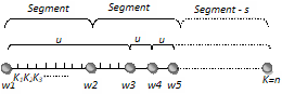
In order for the above to be effected, a simulation environment has been developed using XJ Technologies’ Any Logic simulation tool [19]. The developed environment allows for a UGV of a given propulsion power storage capacity to traverse a predefined route over varying terrains. The simulation allows for the predefined route to be divided into segments, each segment representing a type of terrain of a given rolling resistance. User defined waypoints (w=1…n) at any point in the route define either a change in velocity (u) or a change in terrain. Samples of current, velocity and slip will be taken at intervals, (k= 1…n) of interval length Δt (see Figure 3).
It is assumed that empirical data (to be utilised by the simulation) is collected from sampling terrain as described by Odedra [12], but for three given moisture content conditions (dry, moist, saturated) and at given velocities for all terrain types within the simulation (see table 1). From this, data sets describing current vs. velocity relationships for all terrain types under varying levels of moisture are used by the simulation for prediction. The simulation randomly applies differing rolling resistance values for terrain types (within user defined levels) to simulate unpredicted moisture content of terrain types.
The purpose of the experiments is assessment of methods of prediction for propulsion power usage opposed to power usage of other equipment, so power used is a function of terrain type, current terrain conditions and velocity. Acceleration affects both slip and sinkage but over long mission distances the impact on consumption becomes much less significant so will be ignored here.
The simulation carries out both an offline and online prediction. The offline prediction of propulsion energy requirements is based on empirical data and prior knowledge only. Following from this, the online prediction uses current sensor data to assess the prevailing conditions and based on the empirical data predicts future terrains rolling resistance values in order to predict energy requirements for the remainder of the mission.
Offline energy consumption prediction is possible due to the prior information regarding distance between waypoints, desired (predefined) velocities and predicted terrain types (though not necessarily entirely accurate), and can be calculated by integrating instantaneous gross power:
| (2) |
|---|
Where is the total energy required for the mission duration (0 to T). In order to allow for exploitation in a discrete time-step simulation the equation can be expressed in the following discrete form:
| (3) |
|---|
Where is simulation step duration, velocity for sample i, the total simulation steps and the discrete function of (v0,P0...vN,PN) from empirical data. For on-line power prediction and at any moment during a mission the total energy prediction for propulsion can be expressed as:
| (4) |
|---|
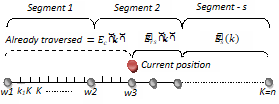
where is total energy required, is energy consumed at point t, is predicted energy for remainder of current segment, and energy required for remainder of whole segments (see Figure 4).
As discussed earlier it is clear that the problem of energy prediction is non-linear by nature. A number of possibilities exist for non-linear analysis to be used in the prediction, however, due to the fact that a particular function presented by the empirical data (and the fact that vehicle/terrain interaction is considered a complex relationship) may have any number of minima/maxima, and the interest is focused on interpolation of the results (opposed to extrapolation) non-Linear Polynomial Regression has been chosen.
By limiting the order of the polynomial the sensitivity to minor changes is reduced. To allow for a point of inflection that is present on some of the empirical data curves, a polynomial of order of three was chosen, which still considers the sensitivity issue.
| (5) | |
|---|---|
| (6) |
Using (5) with empirical data (Table 1) and ordinary least squares estimation (6) where the dimension of a is Energy per velocity, it is possible to generate polynomial curves where is the predicted energy when the UGV is stationary, (dE/dv) is the rate of increase of energy with reference to velocity, (d2E/dv2) rate of increase of with reference to velocity etc. for prediction with 95% confidence levels (standard error) derived from:
| (7) |
|---|
For actual data (x0,y0...xn,yn) from sensor is read via a moving average filter. The length of the filter is a trade-off between reducing the significance of rapid changes such as momentary wheel slip or sensor noise and adequate response to changes in prevailing conditions. The size of the filter is selectable at the start of the mission and maximum accuracy is achieved when the filter is full.
For (future segments of non-traversed terrain types) sensor data (E, v) from the current terrain is compared to the three (dry, moist and saturated) empirical polynomial curves (8, 9) (whose coefficients are of the dimension MLT-1) for the current terrain type. Where (after filtering) the sensor data lies between two of the empirical polynomial curves (10) is used to determine the future segment’s moisture content.
| (8) | |
|---|---|
| (9) | |
| (10) |
Initially considered is the previously suggested prediction method of Sadropor [5], where a comparison is made between a prediction with prior terrain knowledge (type of terrain) and one without. The experiment considers traversal of terrains that are not considered “off-road” but two types of road surface. Sadropors’ method uses linear regression (no prior terrain type knowledge) vs. Bayesian estimation (prior terrain type knowledge).
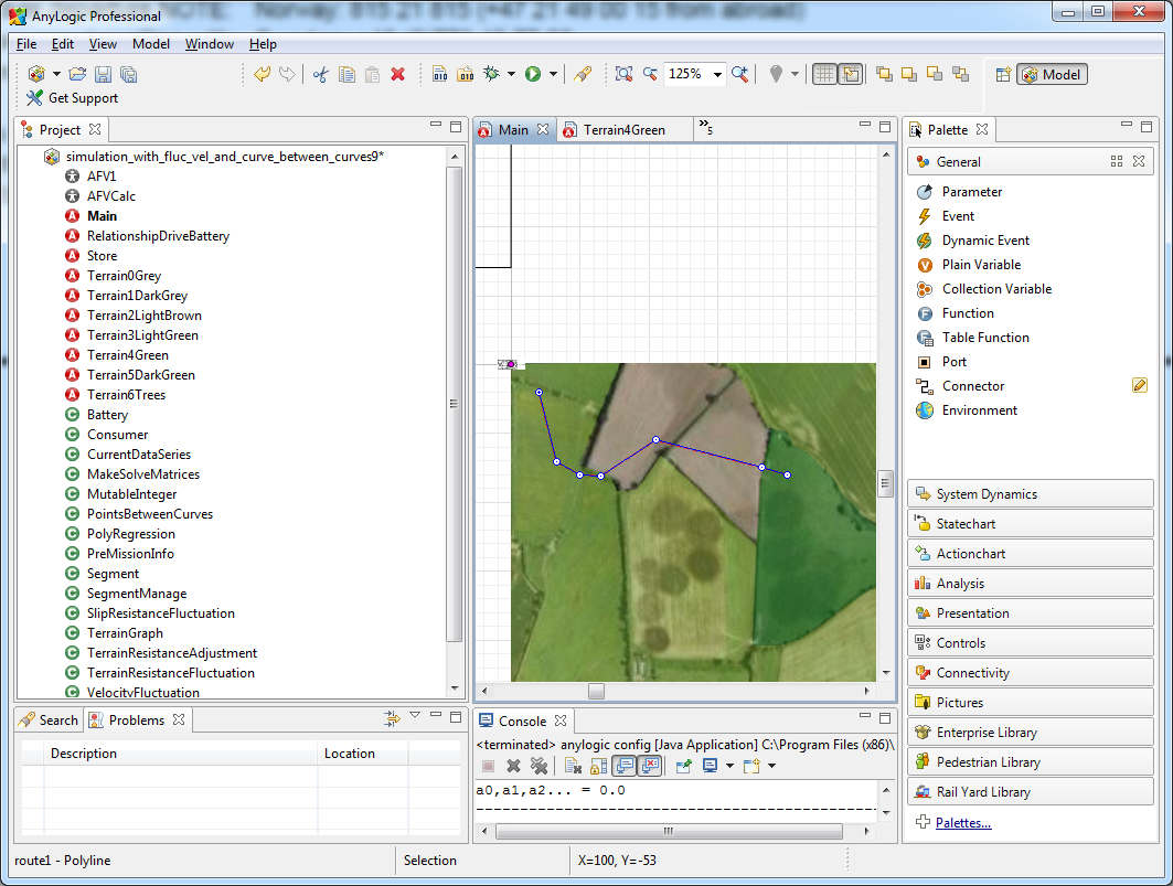
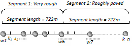
Using empirical data shown in Table 2 and mission parameters shown Figure 5, the simulation provided similar results to that of Sadrpour [5]. The prediction does not take into account the current rolling resistance to enhance the prediction of future terrain rolling resistances. The results in Figure 6 show the prediction with prior knowledge of terrain types does improve overall prediction under the described conditions. It can be seen that the “prediction with no prior knowledge” over-estimates total energy required prior to “w6” being crossed as it assumes that the current rolling resistance will be the same for the remainder of the mission.
| Vel (m/s) | Terrain 0 (KJ) Very Rough | Terrain 1 (KJ) Roughly Paved | ||||
|---|---|---|---|---|---|---|
| dry | moist | saturated | dry | moist | saturated | |
| 1 | 3 | 5 | 6.1 | 4 | 5 | 6.01 |
| 2 | 3.22 | 4 | 6.2 | 3.6 | 4.8 | 5.6 |
| 3 | 3.43 | 3.66 | 6.4 | 3.4 | 4.77 | 5.5 |
| 4 | 3.61 | 4.1 | 6.5 | 3.6 | 5.05 | 5.6 |
| 5 | 4.3 | 4.6 | 6.5 | 4 | 5.81 | 5.82 |
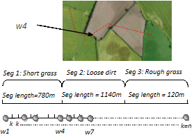
Extending the experiment to consider a range of “off-road” terrains opposed to typical road surfaces reveals obvious shortcomings in the technique in predicting consumption and mission energy requirements, if “off-road” traversal is expected. Using empirical data shown in Table 2 and parameters shown in Figure 7, the UGV traverses other terrain types (whose rolling resistance is affected dramatically by weather conditions) where pre-mission prior knowledge regarding weather effects was inaccurate or incomplete. The prediction does not adjust for un-traversed terrains. Figure 8 shows the results of traversal where actual moisture content for terrains within the simulation are increased by 10% of initial off-line predictions.
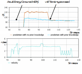
It can be seen that the “prediction with prior knowledge” underestimates energy required until w4 is crossed. Although the prediction takes into account the increased resistance for “Segment 1” it fails to compensate for future terrains.
This is an obvious disadvantage considering the typical deployment of UGV type vehicles on a wide variety of terrain types. Using the same simulation parameters, the implementation of polynomial non-linear regression as described above along with the method of predicting future terrain rolling resistances improved overall prediction as shown in Figure 9. It can be seen that “prediction with prior knowledge” (note that this refers to knowledge regarding terrain type only) prior to crossing w4 under-estimates energy required as no correction is made for future terrain rolling resistance.
It is of importance to note that the prediction methodology assumes that the UGV inclusive of mechanical, electrical and the power/resource management system functions normally. It is assumed that components such as sensors used for collecting data are functioning correctly and no consideration for the monitoring of sensor accuracy is provided. Physical properties of the UGV can also lead to inaccuracies of prediction, for example, during collection of empirical data the tyres of the UGV (assuming the UGV has inflatable tyres) would be inflated to a given pressure, if this pressure were to drop during mission time, the rolling resistance value would be different compared to that of the empirical data collection, resulting in possible inaccurate predictions.
Conclusions
The non-linear function method of consumption prediction introduced here shows improved accuracy of up to 24.2% compared to the previously implemented linear methods for UGV power consumption prediction over a range of off-road terrain types. The previous linear method was shown to provide adequate prediction on finished road surfaces where the problem is considered linear but was proven to be inaccurate when tested over a range of terrain types that are typical of real world UGV operation.
As well as improved prediction of power consumption the non-linear method could indicate future mission terrains’ ability to support mobility of the UGV for the current weather condition. In practice this would provide UGV operators with early warning of any future terrains within the current mission that are likely to be impossible to traverse. This is a significant advantage for UGV missions and would likely improve mission survivability. Improvement in the accuracy of power consumption prediction that considers prevailing climatic conditions and mission terrain types would improve the success rate of UGV missions.
Further work
An important step towards deployment of the non-linear power usage prediction system is to train the system using a physical UGV, over a range of terrain types and weather conditions. This would allow the system to learn real world terrain reference data and the construction of a realistic terrain model library.
Another area for improvement is the inclusion of the effects of incline and wheel slip within the terrain models and prediction algorithm, this would require three-dimensional non linear regression. UGV are subject to a variety of terrain inclination and friction coefficients that will affect power consumption. Future development should account for this.
References
[1] G. Garcia and C.D. Crane, “A Framework for Intelligent Management of Autonomous Ground Vehicle Sensing Resources”, Florida Conference on Recent Advances in Robotics, FCRAR 2010 - Jacksonville, Florida, 20–21 May, 2010.
[2] K. Iagnemma, Mobile Robots in Rough Terrain, Springer-Verlag, Berlin, Heidelberg, p. 1, 2004.
[3] H. Hagras, V. Callaghan, and M. Collry, “Outdoor Mobile Robot Learning and Adaptation” IEEE Robotics & Automation Magazine, Vol. 8, pp. 53–69, 2001.
[4] B. Morley, “Initial Requirements Study into Intelligent Power Management”, 4th SEAS DTC Technical Conference, Edinburgh, UK, 2009.
[5] A. Sadrpour, J. Jin, and A.G. Ulsoy, “Mission Energy Prediction for Unmanned Ground Vehicles”, 2012 IEEE International Conference on Robotics and Automation (ICRA), 2012, pp. 2229–2234.
[6] A.G. Ulsoy, Automotive Control Systems, Cambridge University Press, New York, USA, 2012, p. 57.
[7] J.Y. Wong, Theory of Ground Vehicles, John Wiley & Sons, New York, USA, 2001, p. 11 and p. 92.
[8] M. Spenko, Y. Kuroda, S. Dubowsky, and K. Iagnemma, “Hazard Avoidance for High-speed Mobile Robots in Rough Terrain”, Journal of Field Robotics, Vol. 23, 2006, pp. 311–331.
[9] B. Sofman, J.A. Bagnell, A. Stentz, and N. Vandapel, Terrain Classification from Aerial Data to Support Ground Vehicle Navigation, Robotics Institute Carnegie Mellon University, Pittsburgh, USA, 2006.
[10] S. Zheng and J.H. Reif, “On Finding Energy-minimizing Paths on Terrains”, IEEE Transactions on Robotics, Vol. 21, 2005, pp. 102–114.
[11] A. Sadrpour, J. Jin, and A.G. Ulsoy, “Mission Energy Prediction for Unmanned Ground Vehicles Using Real-time Measurements and Prior Knowledge”, Journal of Field Robotics, Vol. 30, 2013, pp. 399–414.
[12] S. Odedra, “Using Unmanned Ground Vehicle Performance Measurements as a Unique Method of Terrain Classification”, Intelligent Robots and Systems (IROS), 2011, pp. 286–291.
[13] P. Jeary, C. Mellors and D. Ward, “Predictive Traction Power Systems Management for Autonomous Vehicles”, 1st SEAS DTC Technical Conference, Edinburgh 2006.
[14] J.Y. Wong, Terramechanics and Off Road Vehicle Engineering. UK: Elsevier Ltd., Oxford, UK, 15 and 115, 2010, p. 10.
[15] L. Ojeda, J. Borenstein, and G. Witus, “Terrain trafficability characterization with a mobile robot” Unmanned Ground Vehicle Technology VII, Orlando, Florida, USA, 2005, pp. 235–243.
[16] I.C. Schmid, “Interaction of Vehicle and Terrain Results from 10 Years Research at IKK” Journal of Terramechanics, Vol. 32, 1995, pp. 3–26.
[17] S. Odedra, S. Prior, M. Karamanoglu, and S. Siu-Tsen, “Increasing the Trafficability of Unmanned Ground Vehicles Through Intelligent Morphing”, ASME/IFToMM International Conference on Reconfigurable Mechanisms and Robots, 2009, pp. 674–681.
[18] K. D. Iagnemma and S. Dubowsky, “Terrain Estimation for High-speed Rough-terrain Autonomous Vehicle Navigation”, Unmanned Ground Vehicle Technology IV, Orlando, FL,USA, 2002, pp. 256–266.
[19] XJ Technologies. (2014, 20/05/2014). Overview - AnyLogic Simulation Software: http://www.anylogic.com/overview.