
Volume 17, Number 3, November 2014
Effective Solution To The Weapon Target Allocation Problem For Mixed Weapons Using Fuzzy And Optimization Techniques
- 1 Armament Research & Development Establishment, Pashan Pune, 411021 , INDIA.
Abstract
The main objective of the weapon-target allocation problem (WTAP) is to achieve maximum survival of assets and maximum engagement of threats with the minimum number of resources such as weapons, ammunition, and human resources. The WTAP solution space is very large and complex with very large combinations of weapon type, ammunition type and number of rounds to be fired. Within the solution space, there may only be a few local minima and global minima. A very large number of iterations and execution time may be necessary when using conventional methods to identify optimum solutions within the solution space. This paper present a WTAP solution for mixed weapons. The weapon target ammunition data has been generated using Monte-Carlo simulation. An optimum solution has been estimated for a WTAP solution using a fuzzy approach—WTAP-Fuzzy. In addition to WTAP-Fuzzy, WTAP solutions using genetic algorithm (WTAP-GA); particle swarm optimization (WTAP-PSO); and simulated annealing (WTAP-SA) have been simulated and analysed and shown to have similar performance to WTAP-Fuzzy.
Introduction
On the battlefield, a wide range of types of weapons can be distributed over broad frontages and long ranges. In this work, ‘weapon’ refers to the defender’s weapons and ‘target’ refers to the attacker’s weapons. To minimize the battlefield cost an optimum solution to the weapon-target allocation problem (WTAP) is essential. In this paper, a number of mixed weapon types and ammunition types are considered for engaging ground target(s) in the defined mission. A ground target is an area target at any altitude in which a number of targets are distributed around the centre of the target-area. Target engagement is classified as one of three types according to the percentage of target engagement: target annihilation is defined as total destruction of target (that is, over 70% of target engagement); target neutralization as 30% to 70% target engagement; and target harassment as less than 30% target engagement within the target area. Target engagement value is directly proportional to the target hardness value and the number of submunitions that hit the target. The target hardness value classifies the target as soft, medium, or hard.
WTAP is a very complex problem. A number of researchers are working in the area of resource allocation, dynamic WTAP solutions for military forces, using different methods. Rao et al [1] have proposed multi-attribute utility theory for finding utility between alternatives that are characterized by multiple-attributes. In this model, weights are given by analytic hierarchy process to evaluate the weapon system’s static and dynamic combat potential. Simulation has been carried out for army, navy and air force resources and then combined to obtain joint force potentials for a given combat scenario. Tong et al [2] have proposed two methods such as genetic algorithm (GA) and particle swarm optimization (PSO) for the real time strategy (RTS) games to handle the problem of multi-team weapon-target assignment (MT-WTA) and distribution of defensive position with restrictive limit of weapon resources. Initially they have used GA to assign different types of weapons under limited resources and optimal results are applied into a random game’s map to obtain final defensive locations. It is claimed that GA and PSO can be used to achieve the best distribution of defensive positions. Both methods have been compared in RTS Games. It is observed that these two methods have provided efficient, interesting artificial intelligence solutions for real-time strategy games problems. Wu et al [3] have presented an anytime algorithm based on modified GA to solve the dynamic WTAP (DWTAP) in which targets are assigned to weapons one by one as each target enters the launching zone of the weapon. Modified GA is applied to the case in which targets are reduced by continuous interception until all are neutralized—that is, the number of weapons in use decreases over time. Rosenberger et al [4] have extended the basic WTAP by allowing for multiple target assignments per platform, subject to the number of weapons available and their effectiveness. The problem was formulated as a linear integer programming problem and analysed using greedy approach and branch-and-bound methods. Comparison of the two methods has identified that the branch-and-bound technique is feasible to assign multiple platforms per target, and its utility is demonstrated for collaborative asset planning. It is claimed that results herein are readily applicable to sensor tasking and similar resource allocation problems. Schumacher et al [5] have developed a network flow optimization model to develop a linear program for optimal resource allocation. It is observed that the method can be used to generate a “tour” of several assignments to be performed consecutively, by running the assignment iteratively and only updating the assigned task with the shortest estimated time-of-arrival (ETA) in each iteration. They have used variable path lengths to improve overall performance and guarantee computation of feasible paths. It is resulted that the network optimization results in an effective allocation of vehicle resources to the required tasks. This method allows assignment of multiple vehicles to a single target, and multiple targets to a single vehicle. Nygard [6] has described a time-phased network optimization model to produce task assignments for powered munitions. The model is developed to run simultaneously and independently at discrete points in time on all of the munitions, and explicitly assign each to 1) choose to strike, 2) assist in classifying a target, or 3) continue searching. Mukhedkar et al [7] have developed a WTAP solution using one type of weapon (W1 or W2) and ammunition (Ammn1) on a target (Tgt1). Target hardness of other targets (Tgt2, Tgt3) has been defined in terms of Tgt1. The number of ammunitions of type Ammn2, Ammn3 to be fired are defined in terms of Ammn1. A generalized form of a Takagi-Sugeno fuzzy system has been modelled by Taniguchi et al [8] for model reduction and robust control. A generalized form of Takagi-Sugeno has been presented, which resulted in a reduction in the number of rules. The approach can be used for any dynamic system to optimize rules. Lee et al [9] proposed GA to predict locally optimal offspring and the concept has been applied to WTAP. A comprehensive coverage of different particle swarm optimization (PSO) applications has been described by AlRashidi et al [10]. PSO was used to optimize the reactive power flow in the power system network to minimize power system losses. In optimal power flow (OPF) PSO has been implemented to estimate optimal settings of the control variables such that the sum of all generator’s cost functions is minimized. Combinatorial optimization and statistical mechanics have been introduced in [11]. The connection between thermal system dynamics (statistical mechanics) and multivariate combinatorial optimization has been presented using simulated annealing (SA) features.
In this paper we present a methodology for allocating an optimum number of different types of weapons and ammunitions to be fired using a fuzzy, GA, PSO, or SA approach for soft, medium and hard targets in accordance with the required percentage target engagement.
Weapon: A weapon is a rugged launch structure with a long launching barrel or multiple barrels mounted on a revolving or fixed turret. It has structure traversing / elevating servo mechanism to position towards the line-of-fire, weapon alignment and pointing mechanism for indicating position and attitude of its platform, round(s) firing system to perform firing of selected round(s), human machine interface (HMI) to input fire mission related information and to monitor outputs. The weapon system can be of type ground, aerial, or marine. Ground type weapons are positioned and deployed on the ground—such as man-portable small arms, vehicle-mounted small arms, mortars, tanks, guns, rocket / missile launchers and howitzers. Ground weapons are used to engage target(s) in the air or on the ground or sometimes at sea. Aerial type weapons are deployed in the air—examples include fighter aircraft, helicopters, and UAV shooters. Aerial weapons are used to engage target(s) on the ground, in the air, at sea, and in space, Marine type weapons are deployed on or in the ocean—such as submarines and surface warships. Marine type weapons are used to engage target(s) on the surface of the sea, under the sea, in the air, or sometimes on the ground. The main objective of a weapon is to launch one or more projectiles with ammunition at the required line of fire to achieve the desired target hit and engagement with the required lethality. Weapon performance is dictated by factors such as consistency and accuracy, wear of barrel, alignment and pointing accuracy, coming in to action time, and coming out of action time.
Target: Targets are threats to a defender—that is, they are assets of an attacker, which are to be engaged in the air, in/on the water, or on the ground. A target can be armoured, covered, vulnerable, or soft-skinned and can therefore be classified as soft, medium, and hard. In a battle scenario, targets may be of mixed-type—that is, they may have a combination of hardnesses. Targets may be distributed over the target area which is defined in terms of length and breadth. There can be number of targets in the target area. Each target is defined in terms of its length, breadth, and orientation. Target engagement is defined as annihilation, neutralization and harassment.
Ammunition: Ammunition causes the lethal effect of its chemical as well as kinetic energy on the target. Ammunitions can be of type aerial burst / impact burst which defines its pattern and lethality effect. Ammunitions can be a) illuminating which illuminates target area b) smoke which generates coloured thick wall clouds of smoke for poor visibility to attacker as well as sometimes it is used to establish coloured patterns as indication to defender troops for executing respective actions (for example, red smoke indicates danger zone, and green indicates clear zone) c) submunitions consist of submunitions which individually have a lethality effect on the target and impact with a certain pattern with Mean Area of Effectiveness (MAE).
Accuracy of weapon at the impact point on the target is critical and is measured in terms of the deviation of the Mean Point of Impact (MPI) (that is, the average value of fall-of-shot of rounds fired) from the target centre. Generally, for example, for an unguided artillery projectile, dispersion is quite high which affects the performance of the weapon.
Problem definition
WTAP deals with defining the optimum number of the same type or of mixed types of weapons and ammunition for engaging a specified target in the defined mission. Allocation of weapons and ammunition should be such that it should result in the desired target engagement—that is, with minimum survival value of attacker’s assets and the maximum survival value of own valuable, sensitive, protected assets. Target information parameters are target type, target size (length × breadth), number of targets in the defined target area and the co-ordinate of centre of the target-area.
In this work, different types of weapons W1 and W2 (see Figure 1) are deployed to engage the desired target. Ground targets have been considered for simulation. Ground targets may be an area target in which a number of targets are located around the centre of the target area (shown as ‘+’ sign in Figure 1(b)). The footprint of rounds fired on the target is shown in Figure 1(c). Footprints on the target dictate damage to the target, which is classified in three types according to the percentage of target engagement. Target annihilation has been defined as total destruction of target with over 75% of target engagement, target neutralization with 30–75% target engagement, and target harassment as less than 30% target engagement within the target area. The target engagement value depends on the target hardness and the number of submunitions hitting the target.
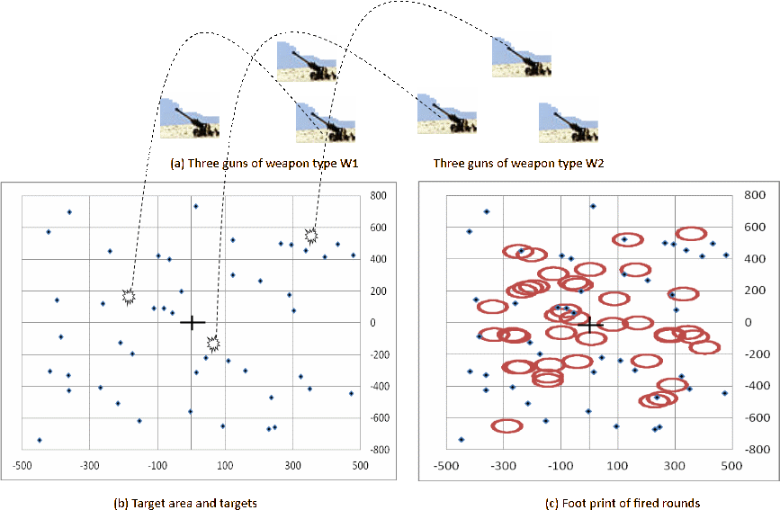
Deployment of different weapon-ammunition combinations are described as follows:
The allocation and deployment of ki number of shooters of weapon type i is as given:
The number of rounds, N, to be fired from i type of weapons, j type of ammunition on target type L is expressed as:
where αi is the number of shooters of weapon type i, and βij is the number of rounds to be fired from the ith weapon and of jth ammunition type.
In this paper, the problem has been formulated for (5) to minimize the total number of rounds to be fired, N, to achieve desired the target engagement, Te, in a combat scenario involving given weapon, target, and ammunition parameters. Target engagement value can be considered in the neighbourhood of Te as Te+ε. Target types are soft, medium and hard.
The objectives of the paper are to develop (a) the WTAP-model, and (b) controlled/optimized mixed weapon deployment and allocation. For a given mission, the WTAP solution with different types of weapons is developed using the fuzzy approach and optimization techniques as GA, PSO, and SA. The procedure for solving the problem with a number of targets, weapons and ammunitions is described here in detail.
Wtap solution using mixed-weapons
The WTAP-solution is necessary to support defenders for the engagement of threats / targets during a combat scenario. A target is defined by its hardness value and the required percentage of engagement—that is, harassment, neutralization, or annihilation.
A weapon-target-ammunition table for mixed-weapons has been generated to provide the input data to WTAP to estimate the number of rounds to be fired against target type of a certain hardness value with a certain percentage of target engagement required.
As an example, deployment of two different types of weapons, W1 and W2, are considered for the mission.
The N rounds to be fired from i=2 types of weapons, with j types of ammunition on target type L is expressed as:
For example: three shooters of W1 and four shooters of W2 are deployed. Two rounds are fired of type j=2 from W1 and three rounds of type j=3 are fired from W2. The total number rounds to be fired can be expressed as:
where α1=3, α2=4, β12=2, and β23=3, therefore total number of rounds fired is (3×2+4×3=18).
Weapon-target-ammunition relation table generation
Weapon-target-ammunition relation tables for mixed weapons have been generated for Ammn1, Ammn2, and Ammn3 fired on soft, medium, hard targets by using Monte Carlo simulation with the following inputs:
a) Maximum number of shooters of same type or mixed type.
b) Maximum number of rounds and ammunition type to be fired from each shooter.
c) Target area (length × breadth).
d) Number of targets in target area, nt.
e) Fired range
f) Range and line consistency of the weapon with respect to the fired range.
g) Range and line accuracy of the weapon with respect to the fired range.
h) Target type (soft, medium, and hard).
Wtap simulation
Simulation is carried out for number of types of ammunition fired from each weapon for target area consisting of targets. The assumptions are used as follows:
a) Gun-bias value is assumed to be zero.
b) The same type of targets are uniformly distributed in target area.
c) Consistency is in terms of Probable Error (PE) as line and range in percentage of fired range.
d) Errors follow a normal distribution.
e) Sub-munition footprint of each round is elliptic.
f) Twenty hits of submunitions on a soft target decides annihilation, on medium decides neutralization, and on hard target decides harassment.
g) Thirty hits of sub-munition on soft target or medium decides annihilation, on hard target decides neutralization.
h) Forty hits of sub-munition on soft, medium, or hard target decides annihilation.
Case study for wtap simulation
Simulation is carried out for fired ammunition of type Ammn1, Ammn2 and Ammn3 from weapons W1 and W2 on to target type soft, medium and hard to generate weapon-target-ammunition relation tables (Table 1, Table 2 and Table 3) with the following assumptions:
i) 1 to 3 guns.
ii) Numbers of rounds fired from each gun are 3, 6, 9, 12 with Ammn1, Ammn2, and Ammn3.
iii) Target area 500m x 500m.
iv) Number of targets 30.
v) Target type: soft, medium and hard.
vi) Target length: 3.5m.
vii) Target width: 3m.
viii) Fired range: 10,000m, 13,000m and 16,000m.
ix) Range, line consistency of W1 is 0.5% and W2 is 0.75% of fired range.
x) Range, line accuracy of W1 is 0.5% and W2 is 0.75% of fired range.
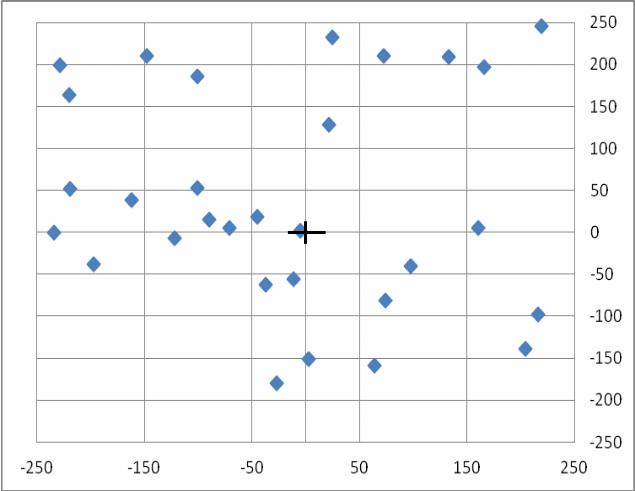
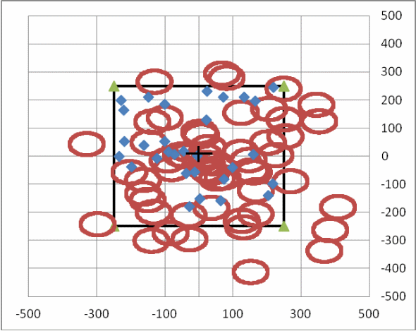
Target area is generated (Figure 2). For two types of weapons W1 and W2 having three guns each and nine rounds are fired from each gun. The elliptic footprints of these 54 rounds are generated with MAE 50m × 40m (Figure 3).
Simulation output data is number of rounds (nr) to be fired from W1+W2 guns (Table 1, Table 2, and Table 3) against an average percentage of target engagement value for soft, medium and hard targets at 10,000m and 13,000m. The value of the average percentage of target engagement against 12 rounds of W1+W2 is derived from target engagement value due to a) three rounds from W1, nine rounds from W2 b) six rounds from W1, six rounds from W2 and c) nine rounds from W1 and three rounds from W2.
Average percentage target engagement value (APTEng) against nr rounds of W1+W2 is defined as:
where αi is the number of shooters (1 to 6) of weapon type i, and βij is the number of rounds (3, 6, 9, 12) to be fired from the ith weapon and of jth ammunition type.
The TEng function is defined to estimate target engagement value for total rounds from W1 and W2. The NC function gives the total number of combinations for nr rounds which satisfies .
For example, for nr = 12, the total combinations can be:
c1 = α1(1)×3+ α2(1)×9 =1×3+1×9=12
c2= α1(1)×3+ α2(3)×3=1×3+3×3=12
c3= α1(1)×6+ α2(2)×3=1×6+2×3=12
c4= α1(1)×6+ α2(1)×6=1×6+1×6=12
c5= α1(1)×9+ α2(1)×3=1×9+1×3=12
c6= α1(2)×3+ α2(1)×6=2×3+1×6=12
c7= α1(2)×3+ α2(2)×3=2×3+2×3=12
c8= α1(3)×3+ α2(1)×3=3×3+1×3=12
where α1(2) means two shooters of W1 and α1(2)×3 means three rounds are fired from each of two shooters of W1.
That is, the total number of combinations NC=8. Thus, the average percentage target engagement for nr = 12 can be estimated as:, where i = 1 to 8, and TEng(1×3+3×3) means the estimated percentage target engagement value for three rounds from one shooter of W1 and three rounds each from three shooters of W2.
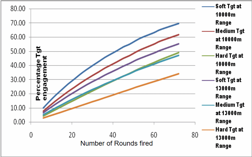
Figure 4 shows the percentage target engagement as a function of the number of rounds required of ammunition type Ammn1, illustrating that the number of rounds required is proportional to the percentage target engagement. A similar result is observed for ammunitions Ammn2 and Ammn3.
Wtap-fuzzy
This section describes the fuzzy approach for the WTAP solution to estimate optimum number of rounds to be fired with deployment of two types of weapons.
Following are the steps to estimate the number of rounds to be fired by using the WTAP Fuzzy Model.
Step 1:
a) WTAP data generation: Monte Carlo Simulation
i) Weapon-Target-Ammunition Table for mixed-weapon (W1+W2).
ii) Target engagement value as a function of the number of guns deployed of (W1+W2) and the number of rounds fired from Ammn1, Ammn2 and Ammn3 on soft, medium and hard targets.
b) Define Triangular Fuzzy membership function for soft, medium and hard targets.
Step 2:
Input: required percentage target engagement (0 to 100), firing range (10,000m to 13,000m), and target hardness value (0 to 100)
Step 3:
a) To estimate the number of rounds of Ammn1, Amnn2 and Ammn3 to be fired to achieve required target engagement for soft, medium and hard targets.
b) Fuzzy Inference Engine: Fuzzification of given crisp input of target hardness value and to estimate membership value in the respective membership function.
i) Estimate fuzzy membership value using algorithms (Algo1 to Algo5 as given below) for given target hardness.
ii) De-fuzzification provides the percentage of soft, medium and hard targets.
iii) Crisp fuzzy output in terms of target hardness value.
Step 4:
WTAP-Fuzzy Output: number of rounds of Ammn1, Ammn2 and Ammn3 to be fired for a given target hardness value in terms of the fuzzy output value.
Fuzzy membership function
Figures 5–8 have been defined for Weapon Target relation as a triangular fuzzy membership function of weapon type W1 and W2. Target types are defined as per target hardness from 0% to 100% for W1 and W2.
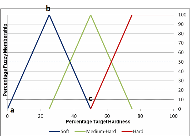
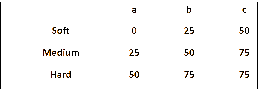
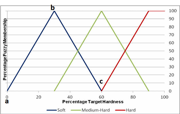
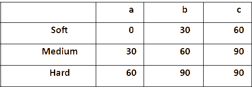
For W1 and soft target, the membership function corner values for 'a', 'b' and 'c' are assumed to be 0, 25 and 50. For W2 those values are 0, 30, and 60. The values represent percentage target hardness on the x-axis. Similarly percentage membership from 0% to 100% membership is represented on the y-axis
Targets are assumed to be soft, medium, or hard. Percentage fuzzy membership value of the given target is estimated depending on the given target hardness input.
Simulation was then carried out with the above defined Weapon Target relation membership functions.
Wtap-fuzzy algorithms
Five algorithms have been defined as follows.
Input:
a) Percentage target engagement value (0 to 100).
b) Firing range in metres (10,000m to 13,000m).
c) Target hardness value.
Algorithm 1:
a) Membership value, mfij, for given inputs, which is estimated for target type (soft, medium, hard) j and weapon type i with respect to weapon-target triangular membership function and given target hardness value.
b) mfij maximum membership function value using ‘OR’ fuzzy operator:
Output:
Estimation of number of rounds Nr(k) of k ammunition types (that is: Ammn1, Ammn2, and Ammn3) to be fired, which is estimated by referring weapon-target ammunition relation table for desired percentage target engagement from corresponding weapon and ammunition type.
where nr(k) is the number of rounds of k ammunition types (that is: Ammn1, Ammn2, and Ammn3) to be fired for full membership value of the target for which maximum membership was found in step b).
The defined model gives optimum (minimum) number of ammunition(s) to be fired from weapon(s) as compared to conventional method of full membership for the target.
Step1 of each algorithm as given below describes estimation of weighted membership factor. Step 2 is common to all Algorithms 2 to 5.
Algorithm 2
In this algorithm, weighted membership factor has been estimated. The estimated weighted value represents continuous target type value.
Weighted membership factor Xi: For given fuzzy input of target hardness value, target type membership function value mfij is estimated for each weapon by referring to its triangular membership of soft, medium, and hard target.
The weapon-weighted membership factor value Xi for each weapon is estimated by using mathematical expression as follows:
where i=1 to number of weapons, and j=1 to number of targets, and the input fuzzy value is the target hardness percentage value and ‘min’ function selects the lowest/minimum hardness value of the corresponding target type (soft, medium and hard) membership function.
Algorithm 3
In this algorithm, a weighted membership factor has been estimated. The estimated weighted value represents a combination of target type(s).
Estimation of the weapon-weighted membership factor Xi: For given fuzzy input of target hardness value, target type membership function value mfij is estimated for each weapon by referring its triangular membership of soft, medium and hard target.
The weapon-weighted membership factor value Xi for each weapon is estimated by using the following mathematical expression:
for i=1 to number of weapons and j=1 to number of targets, and the input fuzzy value is the target hardness percentage value and ‘max’ function is the highest/maximum hardness value of the corresponding target type (soft, medium and hard) membership function.
Algorithm 4
In this algorithm, weighted membership factor has been estimated. The estimated weighted value represents the combination of target type(s).
Estimation of weapon-weighted membership factor Xi: For given fuzzy input of target hardness value, target type membership function value mfij is estimated for each weapon by referring its triangular membership of soft, medium, and hard target.
The weapon-weighted membership factor value Xi for each weapon is estimated by using the following mathematical expression:
for i=1 to number of weapons and j=1 to number of targets, where input fuzzy value is the target hardness percentage value and ‘min’ function is the lowest/minimum hardness value of corresponding target type (soft, medium, and hard) membership function.
Algorithm 5
In this algorithm, weighted membership factor has been estimated. The estimated weighted value represents combination of target type(s).
Step 1:
Estimation of Weapon-Weighted membership factor Xi: For given fuzzy input of target hardness value, target type membership function value mfij is estimated for each weapon by referring its triangular membership of soft, medium and hard target.
The Weapon-Weighted membership factor value Xi for each weapon is estimated by using the following mathematical expression:
For i=1 to number of weapons and j=1 to number of targets, where input fuzzy value is the target hardness percentage value and ‘max’ function is the high/maximum hardness value of corresponding target type (soft, medium and hard) membership function.
Step 2:
Estimation of number of rounds to be fired of A(m,j) (that is, Ammn1, Ammn2, and Ammn3) on soft, medium and hard targets:
Output:
Estimation of number of rounds N(Wr(i,m,j)) to be fired from each weapon Wi :
for i = 1 to number of weapons (W1, W2) , m= 1 to number of ammunition (Ammn1, Ammn2, Ammn3) and j = 1 to number of target type (soft, medium and hard)
Wtap-fuzzy simulation:
The weapons under considerations are of type W1 and W2. Consistency and accuracy of W1 are assumed as 0.5 and 0.5 respectively. Consistency and accuracy of W2 are 0.75 and 0.75 respectively.
Targets under considerations are defined in terms of its hardness value such as soft 0% to 50% hardness, medium 25% to 75% hardness and hard targets 50% to 100% hardness.
Ammunitions under considerations are of sub-munition type, which consists of total 36/45/54 submunitions in 3 layers. Each layer consists of 12/15/18 submunitions respectively. Its lethal area is assumed to be elliptic with major-axis of 25m and minor-axis of 20m. It is assumed that 20 submunitions are required to engage soft target, 30 for medium target, and 40 for hard target.
Consider the problem of calculating the optimum number of rounds to be fired for given conditions, as follows:
Percentage target neutralization: 30%
Weapons: W1, W2
Ammunition:
Ammn1 (36-submunitions, 12-submunitions /layer)
Ammn2 (45-submunitions, 15-submunitions /layer)
Ammn3 (54-submunitions, 18-submunitions /layer)
Target: soft, medium, hard
Target hardness value: 15%, 30%, 60%, 90%
For 30% target engagement at 10,000m range, the maximum number of rounds required is as in Table 4.
Simulation has been carried out by applying WTAP-Fuzzy model for a) 30% Target engagement b) 15%, 30%, 60%, 90% target hardness values, b) Weapon-Target-Ammunition values for Ammn1, Ammn2 and Ammn3 fired on soft, medium and hard targets. The results are shown in Tables 5 to 8. It is seen that number of rounds required to achieve 30% target engagement using WTAP-Fuzzy model is less than that of without fuzzy model (Table 4).
For the input in Table 5 of 15% target hardness gives:
a) 50% membership value of soft, 0% of medium and 0% of hard target for W1.
b) 60% membership value of soft, 0% of medium and 0% of hard target for W2.
For the input in Table 6 of 30% target hardness gives:
a) 100% membership value of soft, 0% of medium and 0% of hard target for W1.
b) 80% membership value of soft, 20% of medium and 0% of hard target for W2
For the input in Table 7 of 60% target hardness gives:
a) 0% membership value of soft, 100% of medium and 0% of hard target for W1.
b) 0% membership value of soft, 60% of medium and 40% of hard target for W2.
For the input in Table 8 of 90% target hardness gives:
a) 0% membership value of soft, 0% of medium and 100% of hard target for W1.
b) 0% membership value of soft, 0% of medium and 100% of hard target for W2.
Table 9 shows the minimum and maximum number of rounds of Ammn1, Ammn2 and Ammn3 are required to engage 30% targets at 10,000m range, with defined target hardness. It shows that number of rounds to be fired is directly proportional to target hardness.
As per the conventional method in Table 4, it is seen that minimum number of rounds required of Ammn1 is 20 and maximum is 41. With the WTAP-Fuzzy approach, the minimum number of rounds required for Ammn1 is 5 to 20 and the maximum is 11 to 40, depending the target hardness value. For Ammn2, as per the conventional method, the minimum number of rounds required is 20 and the maximum is 31. With the WTAP-Fuzzy approach, the minimum number of rounds required for Ammn2 is 5 to 14 and the maximum is 11 to 30, depending target hardness value. Similarly for Ammn3, as per the conventional method, the minimum number of rounds required is 20 and the maximum is 27. With the WTAP-Fuzzy approach, the minimum number of rounds required for Ammn3 is 5 to 12 and the maximum is 11 to 26 depending on the target hardness value. Thus, the WTAP-fuzzy approach always gives the minimum number of rounds required and hence the minimum number of mixed-weapons are required to engage the target as per the target hardness value.
Wtap-genetic algorithm (ga)
The genetic algorithm (GA) was introduced in the 1970s by John Holland and his colleagues and students at the University of Michigan. GA researchers are motivated by observing principles of genetics and evolution towards reproduction of offspring in biological populations. GA solution concludes the principal of “survival of the fittest” in its huge search space. Over a number of generations, desirable solutions are evolved and remain in the desirable composition of the population. The GA approach has been mathematically formulated and extensively used to solve complex optimization problems. GA can handle both discrete and continuous nonlinear objectives with design constrain function(s).
Genetic algorithms are adaptive approaches which may be used for estimating the optimum solution from the total solution space with a minimum number of iterations and within a short time. It is based on the genetic process of evolution of the biological features of organisms in which, over many generations, natural population evolve from natural selection and survival of best-fit. By using the same biological concept, genetic algorithms estimate the best-fit solution for real-world problems.
In this work, the genetic algorithm approach has been considered to estimate the minimum number of rounds to be fired to achieve the require target engagement. Target area, target types, number of targets in target area, weapon types with its consistency and accuracy values, deployment of weapons, ammunition types, foot print types, foot print sizes, MAE values are considered the same as the WTAP-fuzzy parameters.
In this work, the WTAP-GA technique has been used for estimation of the optimum solution to the number of rounds to be fired in a combat scenario for given weapon characteristics (such as consistency and accuracy), target characteristics (such as target area, number of targets, hardness value, and target size), ammunition parameters (such as type, mean area effectiveness (MAE) value, and foot print pattern).
Wtap-ga algorithm
The GA has the basic steps as selection, reproduction, and best-fit-function evaluation. In this work, initial selection is undertaken randomly. Subsequent selection is undertaken as per the best-fit solution as the iteration progresses. Reproduction is achieved by cross-over and mutation among parents. The best-fit-function is defined as the WTAP-system simulation function which estimates percentage target engagement for given weapon consistency, accuracy, number of rounds of defined ammunition type, number of targets in target area, and MAE of rounds fired.
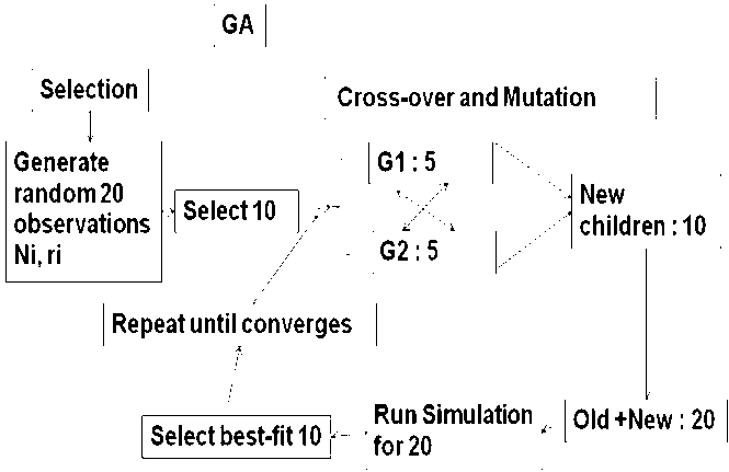
Figure 9 shows a step-by-step GA approach for a WTAP solution, and the pseudo-code for the algorithm is given below in accordance with the above assumptions:
Step1: Randomly generate ns samples for number of shooters for α1 and α2—that is, α1(k) and α2(k) from each W1, W2 respectively, where k=1 to ns and as per the assumption that α1(k) and α2(k) can take any value from 1 to 6.
Step2: Randomly generate ns samples for number of β11 and β21—that is, β11(k) and β21(k) from each W1, W2 respectively, where k=1 to ns and in accordance with the assumption that β11(k) and β21(k) can take any value from 1 to 12.
Step3: Set iterC as 0, where iterC is iteration count
Step4: Compute
N(k)= α1(k) × β11(k) + α2(k) × β21(k)
for each ns samples k=1 to ns and preserve N(k).
Step5: Simulation for ns estimated N(k) values
For k=1 to ns
Percentage_eng(k)= WTAP-Sim(N(k))
Next j
Where WTAP-Sim(N(k)) is a WTP function which estimates percentage target engagement for a given number of rounds to be fired N(k) of specified ammunition type, weapon consistency and accuracy values, size of target area, number of targets in target area, MAE of round fired, foot print pattern of round fired, and target hardness value.
Step 6: Best-fit first ns/2 solutions:
a) Sort above Percentage_eng estimated percentage engagement ns values in ascending order, accordingly update position of N(k)
b) Ignore N(k) and ‘Percentage_eng(k)’ samples for which Percentage_eng(k) are less than desired percentage engagement ‘Percentage_eng’ value and count those ignored observations say ‘ingO’. After ignoring those samples again sort N(k) values as per ‘Percentage_eng(k)’ value.
If ingO > 0 then
icnt=0
while icnt < ingO
generate temporary Ntm(icnt) value randomly and
Estimate Percentage_engTm(icnt) = WTAP-Sim(Ntm(icnt))
If Percentage_engTm(icnt) >= desired_Percentage_eng then
add Ntm(icnt) in to Nr(k) list and Percentage_engTm(icnt) in to Percentage_eng(k)
icnt=icnt+1
if-end
while-end
if-end
c) if ingO > 0 then
Sort ‘Percentage_eng’ array with new additions due to ignored samples in ascending order accordingly update position of N(k).
if-end
d) Select first ns/2 samples from sorted N(k) which are best-fit, where best-fit criteria is acceptance of samples for estimated ‘Percentage_eng’ >= desired_percentage_eng
e) Set Nr_iter(iterC) value as first entry of N(k)
f) Set Percentage_eng_iter(iterC) as first entry of Percentage_eng array
g) Set iterC=iterC+1
(Note: Nr_iter value shows that feasible number of rounds in iteration count iterC and Percentage_eng_iter shows Percentage_eng value of feasible solution of that iteration iterC. The data can be used to plot graphs Nr_ter versus iterC and Percentage_eng versus iterC, which can show multiple local minima which is close to desired target engagement value.)
Step7: Randomly generate two groups G1, G2 of ns/4 samples as Nr1(k) and Nr2(k) from above/last step ns/2 samples, where k=1 to ns/4 and Nr1 of G1, Nr2 of G2
Step8: Cross-over single or multiple
Mcrsovr=1
If mcross = TRUE then // Multiple cross-over
Input Mcrsovr
If-end
While(Mcrsovr>0) //control for single/multiple cross over(s)
For k1 = 1 to ns/4
Select Nr1(k1) value of G1and set to Nt1(k1)
Randomly select k2 from 1 to ns/4
Select Nr2(k2) value of G2 and set to Nt2(k2)
Randomly select value ‘c1’ - 0 to 31 for 32-bit presentation
Swap right ‘c1’ bits among Nt1(k1), Nt2(k2) and
Generate new value of Nt1(k1), Nt2(k2) respectively
Next k1
Mcrsovr=Mcrsovr-1
While-end
Step 9: Mutation single or multiple
Mmutn=1
If mmut = 1 then // Multiple mutation
Input Mmutn // input number of mutations required
If-end
While(Mmutn>0) //Control for single/multiple mutation(s)
For k =1 to ns/4
Randomly select value ‘c1’ - 0 to 31 for Nt1(k) of G1
Mute c1th bit of Nt1(k) :i.e. if c1th bit is 1 make it 0 or 0 make it 1
Preserve new value of Nt1(k)
Randomly select value ‘c2’ - 0 to 31 for Nt2(k) of G2
Mute c2th bit of Nt2(k) :i.e. if c2th bit is 1 make it 0 or 0 make it 1
Preserve new value of Nt1(k), Nt2(k)
Next k
Mmutn=Mmutn-1
While-end
Step10: Data generation for Nr(i2), where i2 = 1 to ns, where first ns/2 are old and next ns/2 are newly generated offspring due to cross-over and mutation
Set i2=1
For k =1 to ns/4
Nr(i2) = Nr1(k) ‘ old of G1
Set i2=i2+1
Nr(i2) = Nr2(k) ‘ old of G2
Set i2=i2+1
Nr(i2) = Nt1(k) //newly generated of G1 due to cross-over and mutation
Set i2=i2+1
Nr(i2) = Nt2(k) //newly generated of G2 due to cross-over and mutation
Set i2=i2+1
Next k
Step 11: Repeat Step6 to Step11 until convergence
Step 12: Declare number of rounds Nrnds to be fired
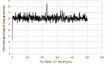
From Figure 10 it is seen that optimal value can be estimated within 300 iterations. Thus WTAP solution can be evolved quickly, which is a basic requirement in a combat scenario.
Generate all possible Combinations for Nrnds with α1, β11, α2, β21 and run simulation for each combination item.
Nrnds= α1 × β11 + α2 × β21
Find the Percentage_Eng for each combination item and find the item which is close to desired_Percentage_eng value
Step13: Declare α1, β11, α2, β21 the best combination item which is close to the desired_Percentage_eng value
In Figure 9 shows, for ns=20 samples, the random selection, cross-over, mutation and best-fit function as a WTAP-Sim function which estimates the percentage target engagement for selected weapon, target and ammunition parameters.
Wtap-ga simulation
WTAP solution has been simulated using above defined GA algorithm with following parameters:
Input:
a) Number of samples ns=20
b) Desire % target engagement: ‘desire_percentage_eng’ = 30%
c) mcross=0, multiple cross over is FALSE (that is, single cross over only)
d) mmut=0, multiple mutation is FALSE (that is, single mutation only)
e) Fired range: 10,000m
f) Range and line consistency: 0.5% of fired range
g) Range and line accuracy: 0.75% of fired range
h) Ammunition type: Ammn1, 12 bomblets/layer
i) Number of targets 20
j) Target length x breadth : 3.5m x 3m
k) Target area: 350m x 350m
l) Target hardness: 30% medium-hard target
The optimum number of rounds to be fired has been estimated by using WTAP-GA as follows:
Output:
a) Total number of rounds required: 23 to achieve 30% target engagement of medium-hard target
b) Number of shooters: 3 each of W1 and W2
c) Number of rounds: 4 of Ammn1 from each shooter
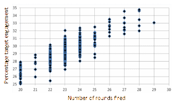
Figure 10 shows the simulation output, number of iterations versus percent target engagement for above given input parameters and defined assumptions. The simulation has been run for 500 iterations. It shows multiple numbers of local minima for desired target engagement value of 30% ± 0.5%.
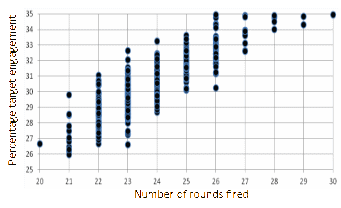
Figure 11 shows number of rounds fired versus percentage target engagement, from which it can be seen that 22, 23 and 24 fired rounds show a maximum coverage from 29.5% to 30.5% for required percent target engagement as 30% ± 0.5%.
Wtap-particle swarm optimization (pso)
Particle swarm optimization (PSO) is a heuristic search method which was invented by Kennedy and Eberhart in the 1990s from swarming or collaborative behaviour of biological population. It is a population-based search method similar to GA. In this algorithm, initial swarm is generated randomly as a set of solutions/particles. As each randomly generated solution has its position and velocity, those solutions are called particles. During each iteration, Particles change their moves towards optimal solution depending on experience and information gained (such as intelligence) by individual particle and collaborative intelligence.
The PSO concept was used for estimating the WTAP solution as a second approach in addition to WTAP-GA. PSO has three steps such as a) generation of the particle’s position and velocity, b) gaining of updated velocity for each particle and c) manoeuvring towards a solution in accordance with individual and collective swarm experience and intelligence in search space. The position and velocity of each particle are vectors. The velocity of each particle is updated as per individual and swarm experience and intelligence with respect to current velocity. The position of each particle is updated as per velocity update with respect to current position. Finally the swarm reaches the optimal solution.
In general, the search space is assumed as D-dimensional, where the ith individual particle can be represented as Xi = (xi1, xi2,…..,xiD) and the velocity of the particle can be represented as Vi = (vi1, vi2,….,viD). In each generation, the best previous experience of the ith particle can be represented as pbesti=(pi1, pi2,….,piD) and gbest is the best global experience of all particles. The velocity and position of each particle is adjusted by:
where i=1 to Ns, Ns-size of swarm, t-iteration step, c1 (self-confidence factor), c2 (swarm confidence factor) are positive constants, r1,r2 are U[0,1] random numbers and Vwt is the velocity weight factor. Vi(t+1) represents updated new velocity with respect to current velocity Vi(t) as first term of above equation. Second term is a ‘cognitive term’ which is the ‘particle’s intelligence’ as personal experience and intelligence towards search space of each particle. The third term is the ‘social term’ which represents ‘collaborative intelligence’ which is collaborative experience and intelligence towards search space in finding the global optimal solution.
For estimating the pbest and gbest parameters, the WTAP-system simulation function ‘WTAP-Sim’ was used. The WTAP-Sim function estimates the percentage target engagement for selected values of weapon consistency, accuracy, number of rounds of defined ammunition type, number of targets in target area, and MAE of rounds fired.
Wtap-pso algorithm
In this work, αi, βij defines a two dimensional space (αi, βij), where αi is the number of shooter of Wi and βij is the number of rounds of ammunition type Aj fired from each shooter of Wi.
As a general term, the total number of rounds fired is as expressed in (5). As an example, two types of weapons W1 and W2 are considered and the same type of ammunition is fired.
The WTAP-PSO algorithm is given below in accordance with the above assumptions:
Step1: Randomly allocate ns observations of (αi, βij), where i=1 to 2 and j=1
Step2: Set t as 0
Step3: Estimate initial Nr(k,t) as
Nr(k,t)= α1(k) × β11(k) + α2(k) × β21(k)
k=1 to ns
Step4: Assume initial V(k,t) is any random velocity k=1 to ns
Step5: Randomly generate r1, r2
Step6: Run WTAP-Sim simulation function for all Nr to estimate percentage target engagement as pbest(k,t)
Step7: Estimate gbest(t) out of pbest(k,t), the best value
Step8: Estimate V(k,t+1) = Vwt×V(k,t) + c1×r1×(pbest(k,t)-Nr(k,t))+c2×r2×(gbest(t)-Nr(k,t)) for next iteration
Step9: Estimate Nr(k,t+1)=Nr(k,t) + V(k,t+1)
Step10: Preserve V(k,t) versus iterC and Nr(k,t) versus iterC
Step11: Set t as t+1
Step12: Repeat Step5 to Step11 until convergence
Step13: Find best Nr whose pbest is close to desire target engagement value
Step14: Find combinations of Nr in terms of (αi, βij), where i=1 to 2 and j=1
Step15: Run simulation for all possible combinations of (αi, βij)
Step16: Declare the best (αi, βij)
Wtap-pso simulation
WTAP solution has been simulated using the PSO algorithm above with the following parameters:
Input values:
a) Number of samples n = 20
b) Desire % target engagement: ‘desire_percentage_eng’ = 30%
c) c1=0.7, c2=0.3, Vwt=0.25
d) Fired range: 10,000m
e) Range and line consistency: 0.5% of fired range
f) Range and line accuracy: 0.75% of fired range
g) Ammunition type: Ammn1-12 bomblets/layer
h) Number of targets: 20
i) Target length x breadth: 3.5m x 3m
j) Target area: 350m x 350m
k) Target hardness: 30% medium-hard target
The optimum number of rounds to be fired can be estimated by using WTAP-PSO as follows:
Output:
a) Total number of rounds required: 23 to achieve 30% target engagement of medium-hard target
b) Number of shooters: 3 each of W1 and W2
c) Number of rounds: 4 of Ammn1 from each shooter
d) Figure 12 shows simulation output, number of iterations versus percent target engagement for the above input parameters and defined assumptions. Simulation shows multiple local minima for desired target engagement value of 30% ± 0.5%.
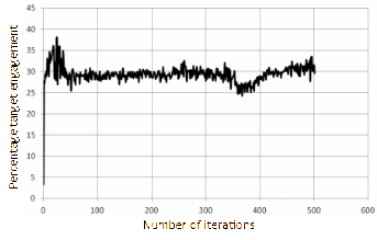
Figure 13 shows the number of rounds fired versus percentage target engagement. It can be seen that for 23 and 24 rounds fired there is a maximum coverage from 29.5% to 30.5% for required percent target engagement of 30% ± 0.5%. From the above figures it can be seen that the results of WTAP-GA and WTAP-PSO are very close.
Wtap-simulated annealing (sa)
Researchers are inspired by annealing analogy of transformation of liquid to its crystalline form by applying controlled cooling temperature until frozen point is reached. Whenever the solid material is heated beyond its melting point to form liquid state and then that liquid is cooled slowly to reach its totally crystalline ordered solid state form which is the annealing. It represents minimum energy state of the system. However, fast cooling results in a nebulous structure having higher energy which represents a local minimum. When the liquid is cooled slowly, the atoms have sufficient time to reach a thermal equilibrium stage during each temperature state. In this state, system obeys the Boltzmann distribution:
where p(E) is the probability distribution of the energy values E as a function of temperature, T, and k is Boltzmann constant. For every temperature value, each energy has non-zero probability, the system can change its state to a higher or lower energy. Lower energy corresponds to local minima and slow cooling reaches a global minimum by crossing multiple local minima.
Simulated annealing (SA) originated in statistical mechanics, formulated for classical combinatorial optimization problems such as the travelling salesman problem (TSP). During the process, SA allows uphill moves which are different from other iterative methods. Normally an uphill move spoils the temporary solution, whereas SA supports an uphill climb in a controlled way. SA is useful for problems with very large discrete configuration space in which very high exhaustive search is required for minimizing or maximizing objective function. The SA procedure is repeated until the termination condition is reached, by which local minima may be identified rather than a global minimum.
Basically SA is based on a neighbourhood search which defines the next neighbouring acceptable feasible move from the current state. An acceptable feasible move is based on a greedy heuristic approach which always moves from the current solution to the best neighbouring solution. During the process, the SA technique crosses local minima and finally reaches a global minimum in a similar manner to a slow cooling process.
In this work, the SA concept has been used for estimating the WTAP solution as another approach in addition to WTAP-GA, and WTAP-PSO.
Wtap-sa algorithm
WTAP-SA algorithm is given below in accordance with the above assumptions:
Step1: Construct initial solution X0, set XNow = X0
XNow = (α1, β11, α2, β21)
estimate N = α1 × β11 + α2 × β21
Step2: Set initial temperature T = TI
Step3: Set TL = number of iterations for each temperature state
Step4: Set epsilon = temperature cooling step
Step5: Set k = 1
Step6: Randomly generate neighbouring solution X’ to N(XNow), N-neighbouring function
X’=(α’1, β’11, α’2, β’21):
estimate N’ = α’1 × β’11 + α’2 × β’21
Step7: Estimate C(X’)=WTAP-Sim(N’), C(XNow)=WTAP-Sim(N)
Step8: Compute change of cost
ΔC=C(X’)– C(XNow)
if then
XNow = X’ (accept new state)
else
Generate random number q = U[0,1]
If then XNow = X’
if-end
if-end
Step9: Set k=k+1
Step10: if k < TL then go to Step6
Step11: Set new temperature T=f(T), where f(T) = T-epsilon
Step12: if T > stop_criteria then go to Step5
Step13: Declare solution corresponding to minimum cost function value as XNow which gives minimum number of rounds to be fired.
Wtap-sa simulation
WTAP-SA simulation was carried out with the following parameters:
Input values:
a) Initial temperature TI = 52
b) Number of iterations at each temperature state: TL =50
c) Temperature cooling step: epsilon = 0.1
d) Stop_criteria = 0, SA process should stop at T<0
e) Desire % target engagement: ‘desire_percentage_eng’ = 30%
f) Fired range: 10,000m
g) Range and line consistency: 0.5% of fired range
h) Range and line accuracy: 0.75% of fired range
i) Ammunition type: Ammn1, 12 bomblets/layer
j) Number of targets: 20
k) Target length x breadth: 3.5m x 3m
l) Target area: 350m x 350m
m) Target hardness: 30% medium-hard target
The optimum number of rounds to be fired has been estimated by using WTAP-SA as follows:
Output:
a) Total number of rounds required: 22 to achieve 30% target engagement of medium-hard target.
b) No of shooters: 3 each of W1 and W2.
c) No of rounds: 4 of Ammn1 from each shooter
d) Results are close to WTAP-GA, WTAP-PSO.
Figure 14 shows the simulation output, illustrating temperature versus percent target engagement for the above input parameters and defined assumptions. The simulation shows multiple local minima for the desired target engagement value of 30% ± 0.5% and a global minimum at a temperature value around 4.
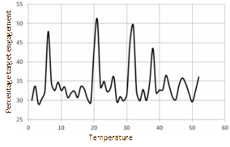
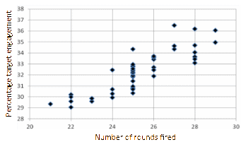
Figure 15 shows the number of rounds fired versus temperature, from which it can be seen that for 22 rounds fired, there is a maximum coverage for the required percentage target engagement of 30% ± 0.5%. From the above figures it can be seen that results of WTAP-SA, WTAP-GA and WTAP-PSO are very close.
Observations
The following observations can be made:
a) WTAP-system is very complex and has a very large discrete search space for estimating optimal solution.
b) The defined WTAP solution model provides a generic solution to generate realistic combat scenarios for given values of weapon-consistency, weapon-accuracy, firing range, target area, target type, and number of targets in target area.
c) The proposed WTAP-Fuzzy, WTAP-GA, WTAP-PSO and WTAP-SA approaches estimate the optimal number of rounds to be fired and the optimum number of weapons to be deployed in a combat scenario.
d) The WTAP-Fuzzy algorithm works as a multivalent logic with percentage truth value and perception.
e) The WTAP-GA, WTAP-PSO, and WTAP-SA are evolutionary heuristic algorithms with a combination of deterministic and probabilistic rules.
f) The WTAP-Fuzzy, WTAP-GA, WTAP-PSO and WTAP-SA minimize economical, logistical, manpower constraint and time regards in combat scenario.
g) The estimated optimum values using WTAP-GA, WTAP-PSO and WTAP-SA are close to those obtained using WTAP-Fuzzy.
h) WTAP-GA is computationally expensive as compared to WTAP-PSO and WTAP-SA.
i) WTAP-GA with multiple-crossover and multiple-mutation gives a slightly better optimal value with very high computational cost.
j) WTAP-PSO defines a set of particles which have position and velocity vectors. Each particle manoeuvres in accordance with its individual and swarm knowledge and intelligence, providing an optimal solution.
k) In WTAP-SA, a small number of iterations in high temperature and large number of iterations in low temperature provides an optimal solution at a faster rate.
l) WTAP-SA supports control of uphill climb.
m) WTAP-Fuzzy, WTAP-GA, WTAP-PSO and WTAP-SA are robust methods that provide optimum solutions in a short time which is the basic requirement in support of a combat scenario.
Conclusions
A combat scenario is usually non-linear and therefore the fuzzy approach to WTAP provide a solution for vague, ambiguous, imprecise, and noisy inputs. As compared to the conventional method, the fuzzy approach to WTAP with mixed weapons always provides a minimum number of rounds to be fired in accordance with target hardness value in the combat scenario.
WTAP-GA, WTAP-PSO, and WTAP-SA also provide estimates of the optimal solution that are close to those obtained using WTAP-Fuzzy. Any one of the above optimization techniques can be used as a WTAP solution in a combat scenario in order to satisfy the requirement for quick robust solution in military applications.
Acknowledgement
We express sincere thanks to Dr K.M. Rajan, Director ARDE for his valuable inspiration.
Biographies
Mr R.J. Mukhedkar received his MSc (Computer Science) and MTech (Modelling and Simulation) from Pune University. He is currently pursuing his doctoral studies at the Defence Institute of Advanced Technology (DIAT) Deemed University (DU), Pune. He is currently a scientist at ARDE, Pune. His research interests include: advanced modelling techniques for military applications, weapon target allocation problem, trajectory correction system, network centric warfare, complex warfare systems modelling and simulation.
Dr (Mrs) S.D. Naik received MSc (Mathematics) and PhD (Applied Mathematics) from Pune University. She is currently a scientist at ARDE, Pune. Her research interests include: Flight Dynamics and allied problems related to Defence. She has over 50 publications in Peer reviewed International Journals/conferences. She has guided 18 MTech and six PhD students. She is a member of Indian Women Scientist’s Association, Indian Mathematical Society, Indian Academy of Industrial and Applicable Mathematics, Indian Society of Industrial and Applied Mathematics. She was awarded the Laboratory Award– Scientist of the year in 2003.
| Number of rounds to be fired from W1+W2 | Soft Target average Percentage Engagement at Range 10,000m | Medium-hard Target average Percentage Engagement at Range 10,000m | Hard Target average Percentage Engagement Range 10,000m | Soft Target average Percentage Engagement at Range 13,000m | Medium-hard Target average Percentage Engagement at Range 13,000m | Hard Target average Percentage Engagement Range 13,000m |
|---|---|---|---|---|---|---|
| 6 | 9.87 | 7.62 | 4.16 | 6.65 | 5.12 | 2.73 |
| 9 | 14.52 | 11.33 | 6.38 | 9.80 | 7.59 | 4.17 |
| 12 | 18.85 | 14.85 | 8.66 | 12.78 | 9.98 | 5.57 |
| 15 | 22.79 | 18.16 | 10.88 | 15.58 | 12.24 | 6.99 |
| 18 | 26.68 | 21.4 | 13.18 | 18.46 | 14.57 | 8.48 |
| 21 | 30.12 | 24.34 | 15.32 | 21.09 | 16.74 | 9.91 |
| 24 | 33.68 | 27.38 | 17.58 | 23.69 | 18.9 | 11.38 |
| 27 | 36.87 | 30.17 | 19.75 | 26.27 | 21.01 | 12.83 |
| 30 | 39.81 | 32.81 | 21.93 | 28.62 | 23.05 | 14.3 |
| 33 | 42.63 | 35.33 | 24.07 | 30.77 | 24.88 | 15.66 |
| 36 | 45.56 | 38.05 | 26.25 | 33.19 | 26.93 | 17.16 |
| 39 | 47.98 | 40.24 | 28.3 | 35.25 | 28.72 | 18.57 |
| 42 | 50.38 | 42.52 | 30.31 | 37.32 | 30.6 | 20.06 |
| 45 | 52.98 | 44.93 | 32.37 | 39.50 | 32.5 | 21.51 |
| 48 | 54.87 | 46.83 | 34.29 | 41.37 | 34.18 | 22.92 |
| 51 | 57.39 | 49.26 | 36.47 | 43.62 | 36.28 | 24.51 |
| 54 | 59.61 | 51.38 | 38.44 | 45.43 | 37.88 | 25.87 |
| 60 | 63.09 | 54.99 | 42.05 | 48.76 | 41.01 | 28.61 |
| 63 | 65.17 | 57.07 | 43.97 | 50.61 | 42.72 | 29.96 |
| 72 | 69.52 | 61.64 | 49.06 | 55.21 | 47.21 | 34.15 |
| Number of rounds to be fired from W1+W2 | Soft Target average Percentage Engagement at Range 10,000m | Medium-hard Target average Percentage Engagement at Range 10,000m | Hard Target average Percentage Engagement Range 10,000m | Soft Target average Percentage Engagement at Range 13,000m | Medium-hard Target average Percentage Engagement at Range 13,000m | Hard Target average Percentage Engagement Range 13,000m |
|---|---|---|---|---|---|---|
| 6 | 10.02 | 8.77 | 6.27 | 6.76 | 5.91 | 4.19 |
| 9 | 14.72 | 12.93 | 9.35 | 9.95 | 8.69 | 6.24 |
| 12 | 19.10 | 16.86 | 12.38 | 12.96 | 11.37 | 8.23 |
| 15 | 23.08 | 20.48 | 15.25 | 15.79 | 13.91 | 10.15 |
| 18 | 27.01 | 24.05 | 18.14 | 18.71 | 16.52 | 12.14 |
| 21 | 30.47 | 27.25 | 20.73 | 21.36 | 18.91 | 14.01 |
| 24 | 34.06 | 30.56 | 23.46 | 23.99 | 21.30 | 15.90 |
| 27 | 37.26 | 33.54 | 26.01 | 26.59 | 23.66 | 17.75 |
| 30 | 40.23 | 36.34 | 28.45 | 28.97 | 25.85 | 19.56 |
| 33 | 43.06 | 39.00 | 30.83 | 31.13 | 27.86 | 21.22 |
| 36 | 46.02 | 41.84 | 33.35 | 33.57 | 30.06 | 23.09 |
| 39 | 48.44 | 44.18 | 35.43 | 35.64 | 32.01 | 24.65 |
| 42 | 50.84 | 46.50 | 37.62 | 37.73 | 33.98 | 26.39 |
| 45 | 53.46 | 49.00 | 39.92 | 39.92 | 36.00 | 28.11 |
| 48 | 55.33 | 50.91 | 41.79 | 41.80 | 37.80 | 29.71 |
| 51 | 57.89 | 53.36 | 44.15 | 44.07 | 39.90 | 31.61 |
| 54 | 60.10 | 55.54 | 46.26 | 45.90 | 41.62 | 33.15 |
| 60 | 63.57 | 59.04 | 49.85 | 49.24 | 44.91 | 36.09 |
| 63 | 65.67 | 61.17 | 51.90 | 51.11 | 46.65 | 37.72 |
| 72 | 69.99 | 65.60 | 56.58 | 55.72 | 51.22 | 42.06 |
| Number of rounds to be fired from W1+W2 | Soft Target average Percentage Engagement at Range 10,000m | Medium-hard Target average Percentage Engagement at Range 10,000m | Hard Target average Percentage Engagement Range 10,000m | Soft Target average Percentage Engagement at Range 13,000m | Medium-hard Target average Percentage Engagement at Range 13,000m | Hard Target average Percentage Engagement Range 13,000m |
|---|---|---|---|---|---|---|
| 6 | 10.12 | 9.37 | 7.36 | 6.83 | 6.30 | 4.93 |
| 9 | 14.86 | 13.77 | 10.96 | 10.04 | 9.26 | 7.33 |
| 12 | 19.27 | 17.90 | 14.38 | 13.09 | 12.10 | 9.64 |
| 15 | 23.27 | 21.70 | 17.60 | 15.94 | 14.78 | 11.83 |
| 18 | 27.24 | 25.44 | 20.77 | 18.87 | 17.54 | 14.11 |
| 21 | 30.71 | 28.77 | 23.64 | 21.55 | 20.06 | 16.21 |
| 24 | 34.32 | 32.21 | 26.63 | 24.2 | 22.56 | 18.33 |
| 27 | 37.54 | 35.30 | 29.38 | 26.82 | 25.03 | 20.38 |
| 30 | 40.52 | 38.18 | 31.96 | 29.21 | 27.31 | 22.37 |
| 33 | 43.34 | 40.95 | 34.47 | 31.38 | 29.39 | 24.17 |
| 36 | 46.33 | 43.82 | 37.14 | 33.84 | 31.70 | 26.20 |
| 39 | 48.75 | 46.21 | 39.32 | 35.91 | 33.72 | 27.93 |
| 42 | 51.15 | 48.57 | 41.58 | 38.01 | 35.74 | 29.79 |
| 45 | 53.79 | 51.15 | 43.98 | 40.21 | 37.85 | 31.65 |
| 48 | 55.65 | 53.02 | 45.86 | 42.11 | 39.68 | 33.33 |
| 51 | 58.22 | 55.52 | 48.27 | 44.38 | 41.87 | 35.38 |
| 54 | 60.44 | 57.69 | 50.38 | 46.23 | 43.63 | 36.98 |
| 60 | 63.89 | 61.18 | 53.99 | 49.59 | 46.94 | 40.07 |
| 63 | 66 | 63.30 | 56.07 | 51.45 | 48.74 | 41.76 |
| 72 | 70.32 | 67.66 | 60.68 | 56.08 | 53.27 | 46.22 |
| Ammunition type | Total number of rounds are required to fire from W1+W2 to achieve 30% target engagement at 10,000m range, without fuzzy model approach | ||
|---|---|---|---|
| Soft Target | Medium Target | Hard Target | |
| Ammn1 36-submunitions | 20 | 26 | 41 |
| Ammn2 45-submunitions | 20 | 23 | 31 |
| Ammn3 54-submunitions | 20 | 22 | 27 |
| Algorithm | Target engagement: 30%, Fired Range: 10,000m,Target Hardness: 15% | |||||||||
|---|---|---|---|---|---|---|---|---|---|---|
| Soft | Medium | Hard | ||||||||
| 36-subs | 54-subs | 72-subs | 36-subs | 54-subs | 72-subs | 36-subs | 54-subs | 72-subs | ||
| WeaponW1 | Algo1 | 5 | 5 | 5 | 0 | 0 | 0 | 0 | 0 | 0 |
| Algo2 | 2 | 2 | 2 | 0 | 0 | 0 | 0 | 0 | 0 | |
| Algo3 | 2 | 2 | 2 | 0 | 0 | 0 | 0 | 0 | 0 | |
| Algo4 | 5 | 5 | 5 | 0 | 0 | 0 | 0 | 0 | 0 | |
| Algo5 | 5 | 5 | 5 | 0 | 0 | 0 | 0 | 0 | 0 | |
| Weapon W2 | Algo1 | 6 | 6 | 6 | 0 | 0 | 0 | 0 | 0 | 0 |
| Algo2 | 3 | 3 | 3 | 0 | 0 | 0 | 0 | 0 | 0 | |
| Algo3 | 3 | 3 | 3 | 0 | 0 | 0 | 0 | 0 | 0 | |
| Algo4 | 6 | 6 | 6 | 0 | 0 | 0 | 0 | 0 | 0 | |
| Algo5 | 6 | 6 | 6 | 0 | 0 | 0 | 0 | 0 | 0 | |
| Maximum: Total rounds from W1+W2 | 11 | 11 | 11 | 0 | 0 | 0 | 0 | 0 | 0 | |
| Minimum: Total rounds from W1+W2 | 5 | 5 | 5 | 0 | 0 | 0 | 0 | 0 | 0 |
| Algorithm | Target engagement: 30%, Fired Range: 10,000m, Target Hardness: 30% | |||||||||
|---|---|---|---|---|---|---|---|---|---|---|
| Soft | Medium | Hard | ||||||||
| 36-subs | 54-subs | 72-subs | 36-subs | 54-subs | 72-subs | 36-subs | 54-subs | 72-subs | ||
| WeaponW1 | Algo1 | 10 | 10 | 10 | 0 | 0 | 0 | 0 | 0 | 0 |
| Algo2 | 5 | 5 | 5 | 0 | 0 | 0 | 0 | 0 | 0 | |
| Algo3 | 5 | 5 | 5 | 0 | 0 | 0 | 0 | 0 | 0 | |
| Algo4 | 10 | 10 | 10 | 0 | 0 | 0 | 0 | 0 | 0 | |
| Algo5 | 10 | 10 | 10 | 0 | 0 | 0 | 0 | 0 | 0 | |
| Weapon W2 | Algo1 | 8 | 8 | 8 | 2 | 2 | 2 | 0 | 0 | 0 |
| Algo2 | 3 | 3 | 3 | 4 | 3 | 3 | 0 | 0 | 0 | |
| Algo3 | 1 | 1 | 1 | 2 | 2 | 2 | 0 | 0 | 0 | |
| Algo4 | 7 | 7 | 7 | 9 | 7 | 7 | 0 | 0 | 0 | |
| Algo5 | 3 | 3 | 3 | 5 | 4 | 4 | 0 | 0 | 0 | |
| Maximum: Total rounds from W1+W2 | 18 | 18 | 18 | 9 | 7 | 7 | 0 | 0 | 0 | |
| Minimum: Total rounds from W1+W2 | 6 | 6 | 6 | 2 | 2 | 2 | 0 | 0 | 0 |
| Algorithm | Target engagement: 30%, Fired Range : 10000m,Target Hardness : 60% | |||||||||
|---|---|---|---|---|---|---|---|---|---|---|
| Soft | Medium | Hard | ||||||||
| 36-subs | 54-subs | 72-subs | 36-subs | 54-subs | 72-subs | 36-subs | 54-subs | 72-subs | ||
| WeaponW1 | Algo1 | 0 | 0 | 0 | 13 | 11 | 11 | 0 | 0 | 0 |
| Algo2 | 0 | 0 | 0 | 6 | 5 | 5 | 0 | 0 | 0 | |
| Algo3 | 0 | 0 | 0 | 6 | 5 | 5 | 0 | 0 | 0 | |
| Algo4 | 0 | 0 | 0 | 13 | 11 | 11 | 0 | 0 | 0 | |
| Algo5 | 0 | 0 | 0 | 13 | 11 | 11 | 0 | 0 | 0 | |
| Weapon W2 | Algo1 | 0 | 0 | 0 | 7 | 6 | 6 | 8 | 6 | 5 |
| Algo2 | 0 | 0 | 0 | 3 | 3 | 3 | 5 | 4 | 3 | |
| Algo3 | 0 | 0 | 0 | 7 | 2 | 2 | 5 | 3 | 3 | |
| Algo4 | 0 | 0 | 0 | 7 | 6 | 6 | 11 | 8 | 7 | |
| Algo5 | 0 | 0 | 0 | 6 | 5 | 5 | 10 | 7 | 6 | |
| Maximum: Total rounds from W1+W2 | 0 | 0 | 0 | 20 | 17 | 17 | 11 | 8 | 7 | |
| Minimum: Total rounds from W1+W2 | 0 | 0 | 0 | 12 | 7 | 7 | 5 | 3 | 3 |
| Algorithm | Target engagement: 30%, Fired Range: 10,000m,Target Hardness: 90% | |||||||||
|---|---|---|---|---|---|---|---|---|---|---|
| Soft | Medium | Hard | ||||||||
| 36-subs | 54-subs | 72-subs | 36-subs | 54-subs | 72-subs | 36-subs | 54-subs | 72-subs | ||
| WeaponW1 | Algo1 | 0 | 0 | 0 | 0 | 0 | 0 | 20 | 15 | 13 |
| Algo2 | 0 | 0 | 0 | 0 | 0 | 0 | 10 | 7 | 6 | |
| Algo3 | 0 | 0 | 0 | 0 | 0 | 0 | 0 | 0 | 0 | |
| Algo4 | 0 | 0 | 0 | 0 | 0 | 0 | 20 | 15 | 13 | |
| Algo5 | 0 | 0 | 0 | 0 | 0 | 0 | 0 | 0 | 0 | |
| Weapon W2 | Algo1 | 0 | 0 | 0 | 0 | 0 | 0 | 20 | 15 | 13 |
| Algo2 | 0 | 0 | 0 | 0 | 0 | 0 | 10 | 7 | 6 | |
| Algo3 | 0 | 0 | 0 | 0 | 0 | 0 | 0 | 0 | 0 | |
| Algo4 | 0 | 0 | 0 | 0 | 0 | 0 | 20 | 15 | 13 | |
| Algo5 | 0 | 0 | 0 | 0 | 0 | 0 | 0 | 0 | 0 | |
| Maximum: Total rounds from W1+W2 | 0 | 0 | 0 | 0 | 0 | 0 | 40 | 30 | 26 | |
| Minimum: Total rounds from W1+W2 | 0 | 0 | 0 | 0 | 0 | 0 | 20 | 14 | 12 |
| W1 + W2 Minimum Ammunitions would be fired against Target Hardness | W1 + W2 Maximum Ammunitions would be fired against Target Hardness | |||||
|---|---|---|---|---|---|---|
| Target Hardness | Ammn1 36-subs | Ammn2 54-subs | Ammn3 72-subs | Ammn1 36-subs | Ammn2 54-subs | Ammn3 72- subs |
| 15% | 5 | 5 | 5 | 11 | 11 | 11 |
| 30% | 8 | 8 | 8 | 27 | 25 | 25 |
| 60% | 17 | 10 | 10 | 31 | 25 | 24 |
| 90% | 20 | 14 | 12 | 40 | 30 | 26 |
| Conventional method as per Table 4 | 20 | 20 | 20 | 41 | 31 | 27 |
References
[1] D.V. Rao and P.K. Mehra “A Methodology to Evaluate Combat Potential and Military Force Effectiveness for Decision Support”, Journal of Battlefield Technology, Vol. 16, No. 1, March 2013, pp. 27–34.
[2] X.-L T.ong, Y. Li, W.-L. Li, and L.Zhang “Optimization Methods for Resources Allocation in Real-Time Strategy Games”, Proceedings of the 2011 International Conference on Machine Learning and Cybernetics, Guilin, 10–13 July, 2011, pp. 507–513.
[3] L. Wu, C. Xing, F. Lu and P. Jia, An Anytime Algorithm Applied to Dynamic Weapon-Target Allocation Problem with Decreasing Weapons and Targets, IEEE, 2008, pp. 3755–3759.
[4] J.M. Rosenberger, H.S. Hwang, R.P. Pallerla, A. Yucel, R.L. Wilson and E.G. Brungardt, “The Generalized Weapon Target Assignment Problem”, 10th International Command and Control Research and Technology Symposium, June 13–16, 2005, McLean, VA.
[5] C. Schumacher, P.R. Chandler, S.J. Rasmussen and D. Walker, “Task Allocation for Wide Area Search Munitions with Variable Path Length”, Proceedings of the American Control Conference, Denver, Colorado June 4–6, 2003, pp. 3472–3477.
[6] K.E. Nygard, P.R. Chandler, and M. Pachter, “Dynamic Network Flow Optimization Models for Air Vehicle Resource Allocation”, Proceedings of the American Control Conference, Arlington, VA, June 25–27, 2001, pp. 1853–1858.
[7] R.J. Mukhedkar and S.D. Naik, “Weapon Target Allocation Problem using Fuzzy Model”, International Journal of Innovative in Engineering & Management, Vol.2, Issue 6, June 2013.
[8] T. Takagi and M. Sugeno, "Fuzzy Identification of Systems and its applications to Modeling and Control", IEEE Transaction on Systems, Man and Cybernetics, Vol SMC-15, No-1, Jan-Feb 1985, pp. 116–131.
[9] Z.-J. Lee, S.-F. Su, and C.-Y. Lee, "Efficiently solving general Weapon-Target-Assignment Problem by Genetic Algorithms with Greedy Eugenics", IEEE Transactions on Systems, Man, Cybernetics, Vol. 33, No. 1, Feb 2003, pp. 113–121.
[10] M.R. Al Rashidi and M.E. El-Hawary, "A Survey of Particle Swarm Optimization Applications in Electric Power Systems", IEEE Transactions on Evolutionary Computation, Vol. 13, No. 4, August 2009, pp. 913–918.
[11] P. Tian, J. Ma, and D.-M. Zhang, "Application of the Simulated Annealing Algorithm to the Combinatorial Optimization Problem with Permutation Property: An Investigation of Generation Mechanism", European Journal of Operational Research, 118, 1999, pp. 81–94.