Empirical Mode Decomposition Applied To Afghanistan Violence Data: Comparison With Multiplicative Seasonal Decomposition

Introduction

Complex data, composed of multiple modes, are inherently difficult to analyze. A prime example of this is the security incidents such as roadside bombs and ambushes, used as one of the prime objects in the analysis of current military operations. For instance, the trends in violence data from the current conflict in Afghanistan are composed of two major sub-trends, namely seasonal variance and a multi-year trend, and a number of factors such as agricultural circumstances and religious holidays that shift from one year to another and are not well reflected in the annual component. The traditional means of separating these components include approaches such as long-term averaging, comparison of cumulative numbers, and seasonal decomposition [1,2].

This paper compares the analysis of violence data from Afghanistan between 2006 and 2012 using seasonal decomposition [2,3] and a novel approach, called empirical mode decomposition (EMD) [4,5]. The latter was proposed for the use with the violence data in [6]. The key difference between the two approaches is that the EMD does not require a priori assumptions about periodicity; instead, it identifies intrinsic modes peculiar to the analyzed data. It also allows for variable period and even aperiodic components. In addition, unlike other approaches, the EMD enables one to retain short-term dynamics, and thus it provides a tool for removing non-stationarities from the time series. The latter is important for instance in order to study non-normal statistical properties of data at short-time (such as daily) scale [7–10]; however, as this paper demonstrates, the correct identification of medium to long-term behaviour can have serious implications in the context of more traditional analysis of warfare data.

This paper extends the initial assessment of the methodology proposed in reference [6]. It focuses primarily on the longer-term dynamics and the differences between EMD and seasonal decomposition for the analysis of these longer-term trends and drivers, in particular in terms of implications for the assessment of violence changes over medium-to-long term (months to years). However, it also briefly comments on the dynamical properties of identified short-term modes.

The paper is organized as follows. First, a brief discussion of violence data is presented in the context of seasonal influences. Then the EMD methodology and the multiplicative seasonal decomposition are briefly summarized. The data are then decomposed using both methodologies. Finally, the differences in the findings and their impact on interpretation are discussed, first for the longer-term modes, and then for the short-term modes identified by the EMD.

Violent incident data in afghanistan

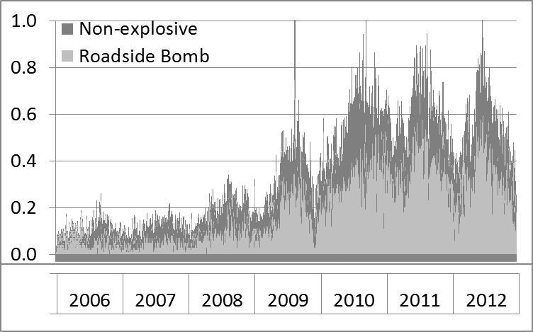
The exact definition of what comprises a security incident can vary somewhat among different organization, but they typically include violent events such as roadside bombs (attempted and exploded), ambushes, raids, anti-aircraft fire, indirect fire incidents, etc. For the purpose of this paper the violent incidents will be comprised of two main groups: roadside bombs (RB), including both exploded bombs and the bombs found and cleared prior to an explosion, and other non-explosive events (NE) including direct and indirect fire incidents and anti-aircraft fire).

Previous studies and analyses [1,2] have shown that the security incident time series are typically composed of multiple trends driven by different mechanisms. Since these different trends are often not easily distinguishable, the overlapping of trends may hide key driving dynamics.

For instance, the trend in violence in Afghanistan (Figure 1) has two major components, seasonal, nearly annual variance and a multi-year trend rendering the time series non-stationary. The seasonality renders determination of causes behind short term increases or decreases difficult. For example, a decline in violence at the end of summer may be simply a seasonal variation, or it may be an actual decline in the enemy capabilities or a will to fight. Which was the case can often be determined only in hindsight, when several more months of data are collected. Methodologies such as seasonal decomposition or EMD attempt to separate trends at different timescales. The stochastic nature of the data limits the applicability of both these approaches in providing immediate answers, since the trends at the very end of a time series can be very difficult to isolate. However, as this paper shows, since the EMD removes the a-priori assumption about the cyclicity of the data, it thus removes the potential artificial relics of the imposed cycles. This provides slightly more reliable long-term trends toward the end of the time series and near turning points.

Seasonal decomposition and emd

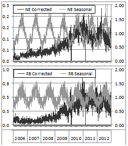
Seasonal decomposition [1,2,3] separates a time series into two factors, a cyclic (seasonal) component, and a long-term trend. The methodology can be summarized as follows. First, the length of the seasonal cycle is determined a priori. The methodology then uses the same period for the entire time series.

A running average of the time series over a single-period duration is calculated. The ratios between the actual and averaged values are then obtained. The values of the cyclic component are calculated as an average of the respective ratios for the same time within period (e.g., for a twelve-month cycle over four years the first value of the cyclic component would be an average of the ratios between real and averaged values for the first, thirteenth, twenty-fifth, and thirty-seventh month). The long-term component is calculated as the ratio of the actual value and the seasonal component.

Figure 2 shows the seasonal decomposition for RB and NE values from Figure 1. The key limitation of the seasonal decomposition is the need to assume the length of the seasonal cycle a priori, and that the length of the cycle remains unchanged over the entire time series. Therefore, its applicability is somewhat limited in the instances when the length of seasonal variations fluctuates, as is the case in Afghanistan violence. However, it can still provide useful insight into the multi-year trend, with the caveat that a caution is required if one is interested in time periods close to peaks and troughs, or towards the end of the analyzed time series.

In contrast, EMD does not require a-priori assumptions about the periodicity of the original time series. The mode basis is defined a posteriori from the decomposition method. The essential idea of EMD is that any time series can be written as the superposition of a small number of signals called intrinsic mode functions (IMFs). These IMFs are obtained iteratively as follows [4,6].

Let {tj} be the local maxima of a signal X(t). The cubic spline E_U (t) connecting the points {(tj, X(tj))} is referred to as the upper envelope of X. The lower envelope E_L(t) is similarly obtained from the local minima {sj} of X(t). Then we define the operator S by:

In the so‐called sifting algorithm, the first intrinsic mode function the EMD is given by:

Subsequent intrinsic mode functions in the EMD are obtained recursively by:

The process stops when Y = X − I₁ − I₂ −…− I_m has at most one local maximum or local minimum. This function Y(t) denotes the local trend in X(t) (long-term trend in the time series).

Since EMD imposes on the data no assumptions about the periodicity of the mode basis, the identified variations are intrinsic to the time series and provide an actual picture of the distinct time scales present in the data.

Results

As is described in the previous section, for the seasonal decomposition, the seasonal variations are assumed a-priori (12 months for the violence data from Afghanistan). Thus, the only calculated component is the long-term trend. Figures 3 and 4 show the rolling 180-day average of the seasonal decomposition for the NE (Figure 3) and RB (Figure 4) incidents. The rolling average was used to eliminate short-term (days to weeks) variations, and to reduce the impact of shifting seasonal minima and maxima in real data. The 12-month seasonal component peaks in July-Sep, and does not provide any significant insights since it was largely imposed on the data. The seasonal cycle is slightly inaccurate, in that while it is the same for each year, in reality the beginning and end of the seasonal increase shifted due to climatic and religious (such as dates for major holidays) factors.

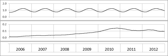
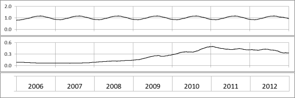
The seasonally corrected component exhibits steady increase between 2006 and 2010; post 2010 it has a slowly declining trend. The initial increase correlates with the increase in the coalition troop strength culminating in the troop surge in 2009–10 and a significant increase in the operational tempo in southern Afghanistan. The saturation and then marginal decline possibly reflect the decline in major combat operations accompanied by the coalition troop drawdown while transitioning the security to Afghan security forces.

The behaviour is fairly similar for both the NE and RB incidents. However, there are some recurrent decreases apparent in RBs which appear toward ends of summer peaks. These are most likely caused by the shift in the actual violence peak toward earlier in a year over time, as the dates for Ramadan and Eid al-Fitr shift. Thus these decreases would be a relic of the methodology rather than an actual trend.

The short-term (daily) variations were removed by averaging. Overall, the seasonal decomposition provides a means to assess the macro-dynamics of the conflict at the longest time scale, but has limited applicability for the assessment of dynamics at medium to short time scales, and of cross-scale behaviour.

In contrast, the EMD did not require prior knowledge of trends or averaging. Nine different intrinsic modes and a residual were obtained (Figure 5 and 7). However, Fourier analysis of the individual modes revealed that some of the modes featured almost identical dominant frequencies and could be grouped together with other modes of a similar frequency. Figure 6 shows a combination of the three low-frequency, strongest modes for the NEs, and Figure 8 shows a combination of the two low-frequency modes for RBs.

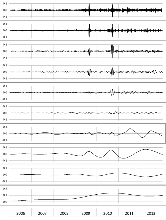
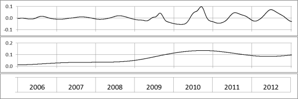
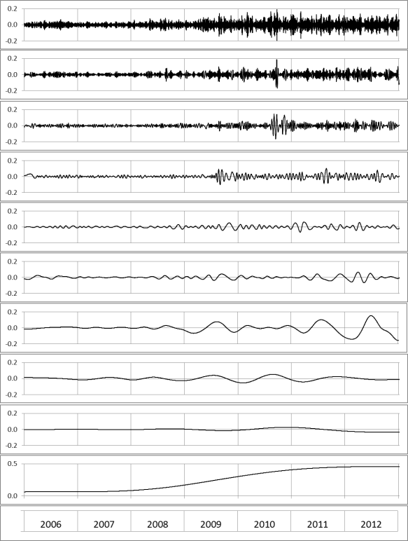
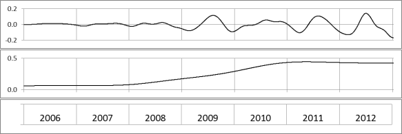
Even a cursory look at the Figures 5-8 suggests that there is no strictly annual (12-month) cycle in the two time series. This was further confirmed using the Fourier analysis on the individual modes as well as on their combination.

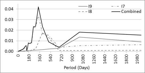
Figure 9 shows the power distribution of the three low-frequency modes (I₇ – I₉). The period for these three lowest-frequency modes range from approximately 11 to 36 months. The longest period is possibly driven by multi-year environmental factors such as alternating severe and milder winters. However, combining these three modes leads to an appearance of a peak corresponding to the period of approximately 12–13 months. For the NEs, the peak is fairly narrow, with a secondary minor peak at approximately 24 months. For the RBs, the peak is wider, ranging from 10–13 months. The secondary increase appears around three-year mark, with noticeable minimum at 24 months.

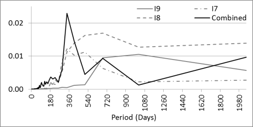
The Fourier analysis of the medium-term modes thus revealed several important points:

• There is indeed a dominant nearly annual cycle in the violence;
• However, the cycle is not strictly 12 months, but can vary between 12–13 months for NEs, and 10–13 months for RBs; and
• There is a distinct difference in the longer-term dynamics between NEs and RBs. While the former have a secondary bi-annual cycle, the latter have slight tri-annual cycle, but no two-year cycle whatsoever.

Point ii) reinforces the limitation of the seasonal decomposition, as it clearly demonstrates that the assumption of strictly periodic time series, with the period of 12 months, is somewhat artificial and can introduce short-term relics in the trends. At the same time the fairly narrow peak in the Fourier spectrum suggests that for the purposes of determining the primary multi-year trend, the assumption is sufficiently reasonable, and the relics can be smoothed out using rolling averages over multiple months.

Point iii) reveals that there is possibly a distinct driver behind the trend in NE and RB incidents. While the detailed assessment of possible drivers and causes is beyond the scope of this paper, one can speculate that it is driven by changes in the operational tempo, shifting relative capabilities between the security forces and insurgents, different dominant means of attack against different force types, and changing target priorities.

There are likely several contributing factors behind the medium to long-term trends. Climatic conditions (winter/rainy season/lack of foliage) are likely the main driver behind the annual cycle. Winter snow in northern and eastern Afghanistan, and heavy rains and a lack of foliage (cover) in the south limit mobility. This impacts fighter and supply availability. Shorter term weather changes (such as days of heavy rains, shorter or later end of winter) and subsequent changes in agricultural seasons (planting and harvest times for variety of key crops, mainly for poppies) are another important factor. The latter, for example, has a significant impact on the availability of local fighters. Coupled with the changes in the dates for religious festivals, since the Islamic calendar differs from the Gregorian calendar typically used in the analysis of Afghanistan data, these factors are probably the main contributor to the changes in the length of the annual cycle.

The long-term, multi-year trend (residual in the EMD) features trend similar to the one obtained using the seasonal decomposition. However, because all shorter-term variations were removed, unlike the seasonally corrected component obtained through the seasonal decomposition, the EMD residual does not contain any short-term variations. This makes it slightly more suited to further analyses.

Qualitatively, the same key drivers behind the long-term trends that were mentioned for the seasonal decomposition apply. In other words, the initial increase correlates with the coalition forces build-up culminating in the surge, leading to the saturation in violence levels which persist until the end of 2012. The similarity is to be expected since the medium trends are similar to the assumed 12 month cycle used for the seasonal decomposition, as was mentioned above.

For completeness, and to demonstrate the capabilities of the EMD, this last part shows analysis of the high-frequency part of the EMD spectrum (with period ranging from days to weeks) (Figures 10 and 11). Even cursory assessment revealed that there was a clear distinction between the NEs and RBs. While NEs had clear dominant periods around 1 week, the high-frequency part of the RB spectrum seemed to drop off with increasing frequencies.

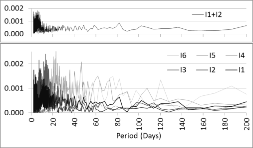
Out of interest, the two highest-frequency modes (I1 and I2; with the main frequencies between 1-14 days) were combined for both incident types (top part of Figures 10 and 11). These combined modes exhibited differences between incident types consistent with the individual modes. While for the NEs the combination of the two high-frequency modes led to fairly solid dominance of a weekly cycle, the RBs exhibited a steady decline in the power with the period.

The difference between the two incident types, notably the lack of weekly cycle for the RBs is possibly caused by the different nature of the attacker-attacked relationship. For the NEs both attacker and defender must be present at the same time (ambush is not an ambush if the attacker or the ambushed is missing). Therefore, if one of the parties exhibits a cycle in its activity (for example, due to religious considerations), the time series will reflect the cycle. On the other hand, the RBs do not require collocation of the attacker and the attacked. In this case, a cycle in the activity of the attacked would drive the overall cyclic behaviour of the time series; while a cycle in the attacker’s activity (such as bomb emplacement) would not. Thus the lack of a distinct pattern is possibly a reflection of the avoidance of friendly forces establishing patterns.

Figure 11 shows the power-frequency dependence for the modes I₃ through I_6. These modes did not have a dominant period; instead, for the high-frequency part of the spectrum, they exhibit behaviour somewhat similar to a 1/f (fractal) spectrum. This is consistent with the power-law frequency distribution of the incidents noted in [11,12].

The high-frequency modes (I₁ and I₂) are behaving in a way typical for white noise, with the power distributed fairly evenly across a wide frequency range (Figure 13). The different scaling of different modes would explain a slight deviation from the power law in reference [12], which used removal of long-term-averaged trend from the data to obtain shorter-term variation.

The random (or pseudo-random) behaviour of the high frequency modes is to be expected. These short term variations are driven by a combination of factors such as weather changes (such as a dust storm lasting several hours can prevent or slow down operations, or an early snowfall or heavy rain can impact the insurgent ability to plant road-side bombs). Since it is impossible to separate all of these factors that in themselves are random, the resulting variations at a sub-day scale should be random as well.

Summary and conclusions

The present paper explores implications of using empirical mode decomposition to deal with complex data sets obtained in the context of irregular warfare, such as violence data from Afghanistan. It compares it to traditionally used seasonal decomposition [1] and identifies limitations of the latter methodology, in particular with respect to an assessment of medium to long-term trends (months to years).

Because it does not impose any a-priori assumptions, the EMD is not a subject to the same limitations as the seasonal decomposition. It enables assessment across all the time scales, ranging from days to years. Using Fourier transforms of the EMD modes of the Afghanistan violence data, the authors identified the presence of several intrinsic time scales present in the data. These included random (pseudo-random) short-term (order of days) variations exhibiting power spectra consistent with the white noise, short-to-medium term mode (weeks to months) with the 1/f power spectrum consistent with the fractal (power-law) size-frequency distribution observed in violence data, medium-to-long term modes exhibiting slightly aperiodic behaviour with the cycle length between 11 and 13 months, and finally a long-term (multi-year) trend exhibiting initial rapid increase correlating with the increased troop density but eventually saturating.

While the seasonal decomposition identified the approximate long-term trend, there were some limitations on assessment due to the a-priori assumption of 12-month cycle in the violence. The variations of the actual cycle from the 12 months assumed by the seasonal decomposition skew the long-term trend in the vicinity of the turning points. This may have adverse effects on fitness of particular functions approximating this trend and consequently on understanding the nature of this variation.

The seasonal decomposition is not suitable to assess shorter-term trends, since unlike the EMD, it effectively imposes the medium-term trend, and averages over the short-term variations.

Overall, the paper demonstrates that the EMD can significantly enhance the analysis of violence data and provide additional insights hidden from other methodologies such as seasonal decomposition. The next step is to use the methodology in the context of different time series in the defence context to demonstrate its validity and usefulness in the overall defence analysis.

References

Author

Peter Dobias received his MSc degree in theoretical physics from the Comenius University, Bratislava, Slovakia and his PhD in physics from the University of Alberta in Edmonton, Alberta, Canada. Currently he works at Defence Research and Development Canada Centre for Operational Research and Analysis. He can be contacted by email at peter.dobias@drdc-rddc.gc.ca, or by phone at +1-250-363-4830.

James Wanliss received his MSc degree in Geophysics from the University Witwatersrand in Johannesburg, South Africa and his PhD in physics from the University of Alberta. He is an Associate Professor of physics at Presbyterian College, South Carolina. His research is in complex systems. He can be contacted by email at jawanliss@presby.edu, or by phone at +1-864-833-7162 or fax at +1-864-833-8993.

References

[1] E. Gons, J. Schroden, R. McAlinden, M. Gaul, and B. VanPoppel, “Challenges of Measuring Progress in Afghanistan Using Violence Trends: The Effects of Aggregation, military operations, seasonality, weather, and Other Causal Factors”, Defence & Security Analysis, Vol. 28, No. 2, 2012, pp. 100–113.
[2] P. Dobias, P. Eles, J. Schroden, and J. Wanliss, “Quantitative Analysis in Support of Military Intelligence: Predicitve Analysis and Risk Assessment in Current Security Environment”, Proceedings from the 28th International Symposium on Military Operational Research, New Place, Hampshire, UK, 28 Aug – 1 Sep 2011 (www.ismor.com).
[3] T. Hill and P. Lewicki, Statistics: Methods and Applications, StatSoft, Tulsa, OK, 2007; (Electronic version: StatSoft, Inc.. Electronic Statistics Textbook. Tulsa, OK: StatSoft, 2012. WEB: http://www.statsoft.com/textbook/).
[4] N.E. Huang, Z. Shen, S.R. Long, M.C. Wu, S.H. Shih, Q. Zheng, C.C. Tung, and H.H. Liu, “The Empirical Mode Decomposition and the Hilbert Spectrum for Nonlinear and Non-stationary Time Series Analysis”, Proceedings of Royal Society of A-Mathematics and Physics, Vol. 454, 1998, pp. 903–993, doi:10.1098/rspa.1998.0193.
[5] V. Anh, Z.-G. Yu, and J.A. Wanliss, “Analysis of Global Geomagnetic Variability”, Nonlinear Processes in Geophysics, Vol. 14, No. 6, pp. 701–708, 2007, doi:10.5194/npg-14-701-2007.
[6] J.A. Wanliss and P. Dobias, “Dealing with Non-Stationarities in Violence Data Using Empirical Mode Decomposition”, Journal of Battlefield Technology, Vol. 16, No. 2, 2013, 16-2-2
[7] J.A. Wanliss and J.M. Weygand, “Power Law Burst Lifetime Distribution of the SYM-H Index”, Geophysical Research Letters, Vol. 34, L04107, 2007, doi:10.1029/2006GL028235.
[8] J.A. Wanliss and V.M. Uritsky, “Understanding Bursty Behavior in Midlatitude Geomagnetic Activity”, Journal of Geophysical Research, Vol. 115, 2010, A03215, doi: 10.1029/2009JA014642.
[9] J.A. Wanliss and M.A. Reynolds, “Fractal Dimension of Low-latitude Geomagnetic Temporal Variations”, Annales Geophysicae, Vol. 21, 2003, pp. 2025-2030, doi: 10.5194/angeo-21-2025-2003.
[10] Z.-G. Yu, V. Anh, Y. Wang, D. Mao, and J. Wanliss, “Modeling and Simulation of the Horizontal Component of the Geomagnetic Field by Fractional Stochastic Differential Equations in Conjunction with Empirical Mode Decomposition”, Journal of Geophysical Research, Vol. 115, 2010, A10219, doi:10.1029/2009JA015206.
[11] P. Dobias, “Self-Organized Criticality in Asymmetric Warfare”, Fractals, Vol. 17, No. 91, 2009, DOI: 10.1142/ S0218348X0900417X.
[12] J.A. Wanliss and P. Dobias, “Fractal Properties of Conflict in Afghanistan Revisited”, Journal of Battlefield Technology, Vol. 15, No. 3, 2012.