Emotional Contagion Theory Applied To Predicting The Result Of Hearts-And-Minds Operations

Introduction

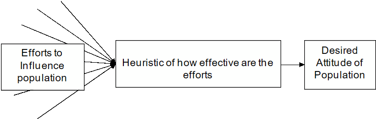
Kilcullen [6] discusses why outsiders have trouble with locals and how locals ‘accidentally’ take up arms against outsiders when there seems to be no logical or rational reason for doing so. We consider the process that influences individuals to oppose outsiders to be part of the phenomenon of spreading processes in social situations that has been formally studied in the mathematics literature since the mid-1920’s. It received particular impetus during the Second World War, the Korean War and the Vietnam War and has occurred throughout recent time and across localities during civil strife, civil wars, police actions, and so on. Work on emotional contagion (Hatfield [5]) and crowd behavior touches on the phenomenon of how ideas and emotions spread. Formal studies have centered on the spread of rumours but, as discussed in Dickinson [2], are applicable to all forms of spreading processes involving social situations or communities. Significant questions are: how many of the population can be expected to be friendly, neutral or hostile at a particular time and, how can this distribution be influenced in one’s favour. Efforts to win over the local population involve civic action such as ‘hearts and minds’ campaigns or, for some, to ensure the lack of action by intimidation. These actions are launched with the heuristic that they will contribute towards the desired result, but how they contribute remains a mystery. Figure 1 illustrates this process.

Regardless of what efforts are made to influence a population this information must be passed within the target population. This can be done by either one or both of a one-to-many or a one-to-one contact process. In this ‘passing’ process an individual of the population will have a reaction on receiving the information. Based on this reaction the individual may or may not change their attitude and spread the information. Over time the attitude of the population will vary as the information spreads. The one-to-one (individual to individual) spreading process in a social situation is likened to contagion. It consists of two aspects—a member of the population’s reaction on being exposed to the information and the behaviour of the population in response to the spread of the information. This paper focuses on the behaviour of the population in response to the spread of the information in a one-to-one contact process.

Using hypothetical probabilities to model an individual’s reaction on being exposed to an effort to influence a population, this paper presents a new method that enables the variation over time of each possible combination of attitudes of the population to be identified. This probabilistic nature of a specific sub-population combination described by the model developed presents the risk associated with a particular strategy. This is markedly different to standard epidemiological models and other models of spreading behaviour which are low fidelity behaviour models presenting the average or expected behaviour of a population, including threshold values to explain why a spreading process which should take off actually dies out.

This paper presents a high fidelity model in which the variation with time of the probability of occurrence of each possible population state from which the expected behaviour of the sub-populations can be derived. These state probability equations render threshold values superfluous, instead giving the probability of occurrence of low probability events such as a spreading process which should die out actually taking off. These state probability equations also demonstrate the existence of the terminal states. By varying the probabilities of an individual’s reaction this paper demonstrates the affect that different strategies and combination of strategies which manipulate individual’s reactions on meeting other members of the same population can have on the desired attitude of a population when faced with a competing attitude.

In discussing this work this paper provides an overview of the general approach to solving a problem in a population for which each member can be in only one of three sub-populations; movement between each sub-population results from a meeting (contact) between two members and this movement between possible states occurs with a known probability (the probability of the individual’s reaction). We consider a staged model with gradual increases in the complexity of the distribution of probabilities for the outcomes of meetings. We conclude with a brief discussion of the usefulness of this method in identifying the effort necessary to create and maintain a friendly population which would inform information campaigns and civic efforts.

General approach

The standard Daley Kendal model in a fixed population, which has been the basis of study to date, is explored in [2]. Consider the case of a population that is composed of three sub-populations: Hostile; Neutral and Friendly. Consider the interaction when two members of the population meet. As the result of the meeting each one could have moved to a different sub-population or remain unaffected. What resultant sub-population they will be in can be stated as a probability which is dependent on the state of the person they meet with and their susceptibility to conversion. These outcomes are represented in the 3×3 matrix at Table 1.

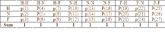
We consider specifically the affect of a pairing on the first member in a pair. In the literature this is what Gani [1] identifies as an α-ρ rumour model. Identifying the probabilities of the reactions of individuals is an area of research in the sociology field. This paper focuses the overall behaviour of the population in response to the spread of the information. Notwithstanding, input values are required to demonstrate the method. In general form these values are represented in the form of Table 2—the probability state matrix for the status of the first member in each pairing at the end of the meeting. Consider the case of a Hostile-Friendly meeting. This is represented in Table 2 as the two columns ‘H-F’ and ‘F-H’. The ‘H-F’ column gives the affect of the meeting on the Hostile member in that they can remain hostile with a probability of P(7), become neutral with a probability of P(8) or become friendly with a probability of P(9). The ‘F-H’ column gives the affect of the meeting on the Friendly member in that they can become hostile with a probability of P(19), become neutral with a probability of P(20) or remain friendly with a probability of P(21). By definition in each column the probabilities sum to unity.

There are many models that can be used to determine the meeting process. Random mixing has been used to date and is used in this paper. Other meeting models are subject to further research. This discussion is based on the communication/meeting between two members of the population being random.

The state of the population is described by the triple (H,N,F). At a particular time t the distribution amongst the three possible sub-populations is given by (h(t), n(t), f(t)) which we abbreviate to (h,n,f). We seek to establish an expression for the probability of occurrence of each combination of the population amongst the three states given an initial state. Following the classical approach for the solution of such a problem the Forward Kolmogorov Equations are derived from the probability state matrix (Table 2). These equations are then expressed in the form of probability generating functions (pgf) which are subjected to a Laplace Transformation. Following the Block Matrix Characterisation of Pearce [8], the block matrices are established. This last step is critical as it allows the probabilities of each sub-population combination to be calculated simultaneously. At this stage of the process we have the ‘Characterisation of the Exact Solution’ of the problem. However, this characterisation is in the form of the Laplace Transform of the solution and, while appropriate mathematically, is not useful in a practical application. The process of inverting the Laplace Transform produces terms in the form of the Dirac Delta function and derivatives of it. As the Dirac Delta function is zero at all points bar the initial conditions; we are given the initial conditions and we desire to know the probabilities of occurrences after t = 0, the terms leading to the Dirac Delta Function can be discarded (see [2]). The probability of occurrence of each state can then be isolated, giving the answer sought.

Theoretically the population size and the number of sub-population categories to which this can be applied are unlimited. However, the calculation of the probability generating functions is a manual process and time consuming. Additionally, the associated calculations are computationally intensive. Using the desk top PC’s analytic solutions to the Daley-Kendal model for populations up to seven have been achieved. This is a significant increase on previous efforts that only modelled a population of two. We discuss techniques for reducing this technological limitation at the end of this paper. In the subsequent discussion a population of six is used for the ease of clarity.

An insurgent model

Returning to a three sub-population model with population elements of Friendly, Neutral and Hostile in which the friendly elements and the hostile elements are competing for the allegiance of the population. We consider that, as the result of the efforts by an outside element wanting to reduce the hostility within the population, the probabilities of outcomes of individual interactions can be manipulated. A number of scenarios are considered reflecting different aspects that can be individually targeted. In all scenarios the start state is an initial population consisting of one hostile, four neutrals and one friendly (1,4,1). For each scenario the probability equations as a function of time for each possible sub-population combination that is a terminal state, the probability of occurrence of each state at t = 10, the expected numbers in each population at t = 10, the graph of the behaviour of the expected values of the sub-populations over time and the final distribution of the populations are presented. At the end the final distributions are consolidated to enable comparison of the result of each scenario.

The selection of the probabilities governing the change of a member of a sub-population is expected to be provided from sociological studies of the population and population sub-groups and do not form part of this paper. Indeed their identification may be problematical and educated best guesses may be necessary. To demonstrate the ability to predict the outcome of efforts to influence a population, the probabilities for a change of sub-population as the result of a meeting used throughout this discussion are chosen arbitrarily.

Scenario 1: unbiased conversion of neutrals only allowed

In the first scenario the friendly subpopulation and the hostile subpopulation are sinks—that is, no conversions from them, and equal effort is applied to converting the neutral population. The probability of outcomes matrix for this model is illustrated in Table 3.

For an initial population of (1,4,1) the probability distributions of the states are given in Table 4.Table 5 gives the complete list of probabilities of occurrence of each possible combination at t = 10.

Thus noting that in this scenario, once becoming hostile or friendly, the population member does not change; the probability that the efforts to convert neutrals to the friendly cause have been successful—that is, a population state of (1,0,5) occurring after 10 time steps, is 3.18%. This is a significant degree of fidelity not available in other models.

The expected numbers in each sub-population at t = 10 are:

• Hostile: 2.39 (40%);
• Neutral: 1.22 (20%); and
• Friendly: 2.39 (40%).

The expected numbers in each of the sub-populations over time is given in Figure 2, which shows the trend for the sub-populations towards the final distribution of:

• Hostile: 3 (50%);
• Neutral: 0; and
• Friendly: 3 (50%).

As both the friendly sub-population and the hostile sub-population are equally attractive then that these numbers are the same is to be expected. However, Table 4 provides the fidelity of the probability of occurrence of each of the terminating states as being:

• Five members of the friendly sub-population and one member of the hostile sub population is 9.7%.
• Four members of the friendly sub-population and two members of the hostile sub population is 24.5%.
• Three members of the friendly sub-population and three members of the hostile sub population is 31.5%.
• Two members of the friendly sub-population and four members of the hostile sub population is 24.5%
• One member of the friendly sub-population and four members of the hostile sub population is 9.7%

Scenario 2: biased conversion of neutrals only allowed

Consider the affect on these proportions if there is a slight change in the attractiveness of the friendly side. In Table 6 the neutrals have been allocated a higher probability of becoming friendly on meeting a friendly member of the population than the equivalent case on meeting a hostile member of the population.

For an initial population of (1,4,1) the probability distributions of the final states are given in Table 7.

Table 8 gives the complete list of probabilities of occurrence of each possible combination at t = 10.

Note that with the change in effort the probability at t = 10 that there will be one hostile, no neutrals and five friendly has increased four fold from 3.18% to 12.87% while the probability of occurrence of opposite state of five hostiles and one friendly is reduced from 3.18% to 1.48%.

The expected numbers in each sub-population at t = 10 are:

• Hostile: 1.93 (32%);
• Neutral: 1.06 (18%); and
• Friendly: 3.01 (50%).

The change in each of the sub-populations over time is given in Figure 3, which shows the trend for the sub-populations towards the final distribution of:

• Hostile: 2.25 (38%);
• Neutral: 0; and
• Friendly: 3.75 (62%).

However, Table 7 provides the fidelity of the probability of occurrence of each of the terminating states as being:

• Five members of the friendly sub-population and one member of the hostile sub population is 32.2%.
• Four members of the friendly sub-population and two members of the hostile sub population is 30.5%.
• Three members of the friendly sub-population and three members of the hostile sub population is 21.4%.
• Two members of the friendly sub-population and four members of the hostile sub population is 11.8%
• One member of the friendly sub-population and four members of the hostile sub population is 4.1%

Hence, though the proportions in the limiting case are not obtainable heuristically, we have a method that quantifies precisely the result for the effort put into targeting the uncommitted members of the population.

If we wish to increase the number in the friendly sub-population; several branches of investigation are available. By varying the attractiveness of the friendly sub-population to the neutral sub-population results in an increase to the friendly sub-population but the community remains polarized as there is no conversion of members of the hostile sub-population.

Scenario 3: introducing an abhorrence factor

Consider introducing an abhorrence factor—when hostiles meet there is a chance that one will be so abhorred by the other’s extremism that they no longer wish to be a hostile, possibly influenced by an information campaign. Hence there is a small probability that the hostile will defect to being a friendly. With balanced outcomes for the neutrals, the probability of outcomes of meetings matrix now becomes as indicated in Table 9.

For an initial population of (1,4,1) the probability distributions of the terminal states are given in Table 10. Table 11 gives the complete list of probabilities of occurrence of each possible combination at t = 10.

With the small change to include the conversion of a hostile we now have a significant change to the previous scenarios. Rather than there always being a hostile remaining after ten time steps we see there is a 0.01% that there will be no hostiles left at all!

To complete the comparison the expected numbers in each sub-population at t = 10 are:

• Hostile: 2.32 (39%);
• Neutral: 1.22 (20%); and
• Friendly: 2.46 (41%).

The change in each of the sub-populations over time is given in Figure 4, which shows the trend for the sub-populations towards the final distribution of:

• Hostile: 0.976 (16.27%);
• Neutral: 0; and
• Friendly: 5.024 (83.73%).

However, Table 10 provides the fidelity of the probability of occurrence of each of the terminating states as being:

• Six members of the friendly sub-population and no members of the hostile sub population is 2.4%
• Five members of the friendly sub-population and one member of the hostile sub population is 97.6%.

We note that while there is now a possibility (2.4%) of ridding the population of hostiles entirely due to an improvement in the prospects of increasing the friendly and the neutral sub-populations from the hostile sub-population, it is remains likely the population will retain a hostile sub-population.

Scenario 4: conversion of hostiles

Another line of investigation is to allow conversions within the two extreme sub-populations. In this next iteration we present a scenario in which an effort has been made to make the friendly side slightly more attractive than the hostile side and hence defections from the hostile occur. The probability of outcomes of meetings matrix now becomes as shown in Table 12.

For an initial population of (1,4,1) a sample of the probability distributions of the states is given in Table 13. Note that as t →∞ it is with a probability of ‘1’ that the population will consist entirely of those who are friendly. Table 14 gives the complete list of probabilities of occurrence of each possible combination at t = 10.

We note that the probability that there will be zero members of the population who are hostile at t = 10 is 0.45%. A small probability, but an increase over the 0.01% of our abhorrence factor consideration.

To complete the comparison the expected numbers in each sub-population at t = 10 are:

• Hostile: 1.28 (38%);
• Neutral: 1.22 (20%); and
• Friendly: 2.51 (42%).

The change in each of the sub-populations over time is given in Figure 5, which shows the trend for the sub-populations towards the final distribution of:

• Hostile: 0;
• Neutral: 0; and
• Friendly: 6 (100%).

This is as given in Table 13 as there is a single terminating state—that of six members of the friendly sub-population and no members of the hostile population with a probability of one. The strategy in this scenario of allowing the conversion of a hostile to a friendly on the meeting of the two results in a final distribution in which there are no members in the hostile sub-population.

Comparison of scenarios and combination of strategies

Table 15 consolidates the figures for the final expected populations of each of the strategies of:

• Scenario 1: Nothing extra is done to make either side attractive to the members of the neutral sub-population (that is, friendly and hostile sub-populations being are equally attractive to the members of the neutral sub-population).
• Scenario 2: An effort is made to make being friendly more attractive to members of the neutral sub-population than being hostile.
• Scenario 3: An effort is made to encourage members of the hostile sub-population to become neutral.
• Scenario 4: Allowing the conversion of members of the hostile sub-population to the friendly sub-population.

A dramatic illustration of the affect of the strategies is demonstrated by expressing the net figures as percentages as is done in Table 16.

Table 17 demonstrates the greater fidelity of this method by consolidating the probabilities of occurrence of each of the terminal states for each of the scenarios. This shows the probability of success (or failure) under the conditions of the scenarios should a particular state be desired. Table 17 demonstrates the affect on the probability of occurrence of manipulating one outcome in the probability matrix of the first scenario. Consideration of the four scenarios together suggests the benefits of each of scenario can be obtained by combining the strategies. A possible combination is demonstrated in Table 18.

While in these scenarios only the movement of a member of the hostile sub-population to the friendly sub-population was considered, such a strategy may be impractical. It may be more practical for the abhorrence factor and the conversion factor to result in a hostile becoming a neutral rather than a friendly. This model provides a mechanism to compare the affect of these different strategies. The amount of effort to be placed into obtaining the probabilities of the outcomes of meetings will depend on the result sought. Objectives such as encouraging a neutral population may be more cost effective than the preferred position of having the population as all friendly, but at the same time one can demonstrate the greater susceptibility of a neutral population to extremism should the effort to retain their neutrality drop off.

Limitations of computing power

More than three sub-populations

In discussing the block matrix approach we noted that additional sub-populations can be added, for example a removed sub-population for those interactions where the hostiles may execute those who do not adopt their cause. This gives the dimensions of the matrices as (M+1)(N+1)*(M+1)(N+1) in which ‘M’ is the number of sub-populations and ‘N’ is the population size. The theory described above is equally applicable to an arbitrary number of sub-populations. Doing so introduces levels of complexity into the calculation of the Forward Kolmogorov Equations as well as demands on computing power.

Dealing with large populations

At first glance the computational implications of dealing with large populations are overwhelming. However, work in the computer sciences, mathematics and sociology, on the clustering of populations, for example Fortunato [4], studies such as Watt’s [9], and the tendency of people to work and socialise within limited groups, lead to the sub-division of the subject population into ever increasing holons. Consider the following hierarchy of holons based on six entities in each holon, the total population of which increases exponentially [2]: Family (six members), Block (six families – 36 people), Neighbourhood (six blocks – 216 people), and so on. Within each grouping, should a threshold number of members be reached, then that group could be considered as being in the appropriate sub-population. Alternatively, the groupings can be treated as a unit of population with the ability to drill down.

Conclusion

In this paper a method of calculating the distribution of a population given an initial state and a probability of outcomes from the meeting of two members of a population has been given. Such is envisaged to be useful in determining a stratagem to create either a neutral or sympathetic population. It would also help determine how much effort should be put in to creating and sustaining the desired sub-population balance.

Areas of further research

This paper used the current practice of presuming a stochastic formation of pairs. The affect of other mixing paradigms is an area of further investigation. It was noted that the selection of the probabilities governing the change of a member of a sub-population may be problematical and educated best guesses may be necessary. It is also standard practice to presume that the probability of the outcome of interactions remains constant throughout the whole process. However, it is likely that as the numbers of hostiles reduce those remaining will become more difficult to change. The investigation of models in which the probability of the outcome of the interactions is dependant on the numbers in each sub-population is an area for future research. Finally the demand on computing power of the described process is great and methods of reducing and/or meeting these demands are areas of research.

References

Author

Rowland Dickinson is employed in the Defence Science and Technology Organisation and has a PhD (University of Adelaide) in the area of stochastic social processes. He has undergraduate degrees in Science (UNSW – Hons Adelaide) and Arts (Ancient History, Pure Maths & Statistics UNE). He has a continuing cross disciplinary interest in military history and mathematics.

References

[1] D.J. Daley and J. Gani, Epidemic Modelling: An Introduction, Cambridge University Press, Cambridge, 1999.
[2] R.E. Dickinson, The Exact Solution to the Stochastic Spread of Social Contagion—Using Rumours, PhD Thesis, University of Adelaide, 17 December 2007.
[3] M. Edwards, A Brief History of Holons, http://www.integralworld.net/edwards13.html accessed 3 November 2010.
[4] S. Fortunato, Community Detection in Graphs, arXiv:0906.0612v1, 2009.
[5] E. Hatfield, J.T. Cacioppo, and R.L. Rapson, Emotional Contagion, Cambridge University Press, Cambridge, 1994.
[6] D. Kilcullen, The Accidental Guerilla: Fighting Small Wars in the Midst of a Big One, University of Oxford Press, New York 2009.
[7] A. Koestler, The Ghost in the Machine, London: Hutchinson, 1990 reprint edition, Penguin Group, 1967.
[8] C.E.M. Pearce, The Exact Solution of the General Stochastic Rumour, Mathematical and Computer Modelling, 31, 2000, 289–298.
[9] D.J. Watts, Six Degrees: The Science of a Connected Age, W.W. Norton & Company, New York, 2003.