
Volume 15, Number 3, November 2012
Fractal Properties Of Conflict In Afghanistan Revisited
- * DRDC CORA, 101 Colonel By Drive, Ottawa, ON, K1A0K2, Canada.
- ** Department of Physics, Presbyterian College, Clinton, SC, 29325 USA.
Abstract
Previous research shows that security incidents in an asymmetric conflict (counter-insurgency, war on terror) exhibit power-law behaviour in terms of casualties and incidents. This study, covering a significantly larger data set than the previous works, confirms the general findings of these earlier analyses. However, it appears that the daily incident counts obey power law distributions only for values greater than the value expected from corresponding monthly average count. The low counts seem to be driven by a completely different mechanism. The present paper proposes that this behaviour is consistent with a dynamical model of insurgency based on a time-dependent Hamiltonian system with a slow free energy (for the insurgency corresponding to their supplies and morale) build-up, followed by a rapid, avalanche-like release. Then the asymmetry in the behaviour for low and high counts can be accounted for as follows. The high counts redistribute the free energy in the form of avalanches of violent incidents (akin to explosive instabilities in many physical systems). On the other hand, the low counts correspond to introducing artificial energy sinks in the system (for example, by localized disruptions to the enemy supply chain or weather-related obstacles). The findings and the model seem to be in line with the studies suggesting that self-organized criticalities form a universality class, opening the door for modeling and possible predictive analysis.
Introduction
Previous research [1,2] shows that security incidents in an asymmetric conflict (counter-insurgency, war on terror) exhibit power-law behaviour in terms of casualties and incidents. Later studies demonstrate that the incident data are often intermittent [3], behaving as fractal point processes, and persistent (self-correlated) [4]. The former result implies that the conflict often develops in surprising or unexpected directions. The latter implies that there is nevertheless a certain pattern that emerges from the broad statistical behaviour. While the above works point out how asymmetric warfare behaves much like a complex system in self-organized criticality, something akin to avalanches on a snowy mountain, all of the previous works are severely limited by small data sets (only up to 18 months of incidents).
In previous papers by the authors, mid-2009 was the cut-off for available data. Now there are three more years of data. Consequently, it is possible to conduct more conclusive analyses. In addition, with more data we are able to examine the possibility that the troop surge in 2009–10 might have shifted conflict dynamics. These two factors are the primary motivation behind the present study.
The paper is organized as follows. First, general trends in the data are discussed. Then the scaling properties of daily incident counts are analyzed, followed by the discussion of persistence in these counts. Last, we discuss relationships between incident and casualty counts and compare these to the findings in [2].
Violent incident data in afghanistan
Violent incidents in Afghanistan can be divided into two main groups: roadside bombs and other kinetic actions. Both feature similar long-term behaviour, including annual cycles with increases in summer and decreases in winter (Figure 1) [5,6]. There is also a multi-year trend (near exponential increase between 2007 and 2010, almost stationary since).
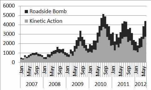
These trends present a challenge when analyzing scaling and self-correlation properties. There are several approaches of dealing with them; for example the seasonal variation can be removed using seasonal decomposition [7]. The multi-year trend is generally more difficult to deal with. It can be removed using, for instance, higher-order polynomial approximations. For the purposes of this paper, two different approaches were used, one for the analysis of scaling properties and a different one for the analysis of persistence.
In order to facilitate the analysis of size-frequency scaling for daily incident counts, the trends were removed via fairly simple methods; the daily incident counts were normalized using monthly counts as a benchmark:
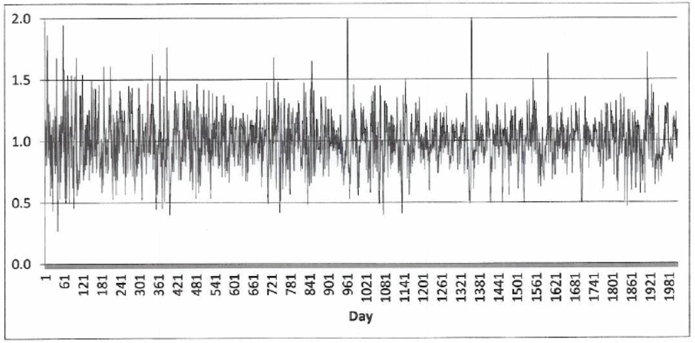
In (1), Dnorm is the renormalized daily count, Ndaily is the number of incidents on a given day, and Nmonthly is the number of incidents and M the number of days in the corresponding month. Figure 2 shows the temporal dependence of renormalized daily counts; the values fluctuate within a fixed band, as is required for the analysis.
Detrended Fluctuation Analysis (DFA) was used to determine the persistence in the data; this approach provides a robust methodology to deal with the trends, as is described below.
Scaling properties of daily incident counts
To identify scaling properties of daily incident counts, the values were renormalized using a multiplicative constant (20 for kinetic action, 40 for roadside bombs, and 25 for total incidents) and rounded to the nearest integer in order to cover a range of approximately 1–100. This facilitates easier calculations without affecting results, because the multiplicative factors become an additive constant when one constructs log-log plot of the normalized number of incidents N versus the number of days DN with at least Nmonthly × N incidents.
There were two distinct regimes identified in the log DN versus log N (Figures 3 and 4), one for low and one for high daily incident counts. For the purpose of this paper low was defined as less than the median renormalized Nmed. Median was chosen over mean (equal to the multiplicative constant), since for symmetric distributions the two coincide, but for skewed, fat-tailed distributions the mean can underestimate the most likely values). The Nmed was determined to be 19 for kinetic action, 39 for roadside bombs, and 24 for total number of incidents.
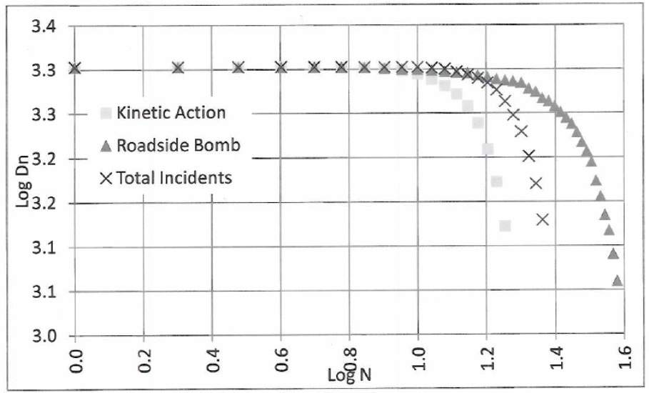
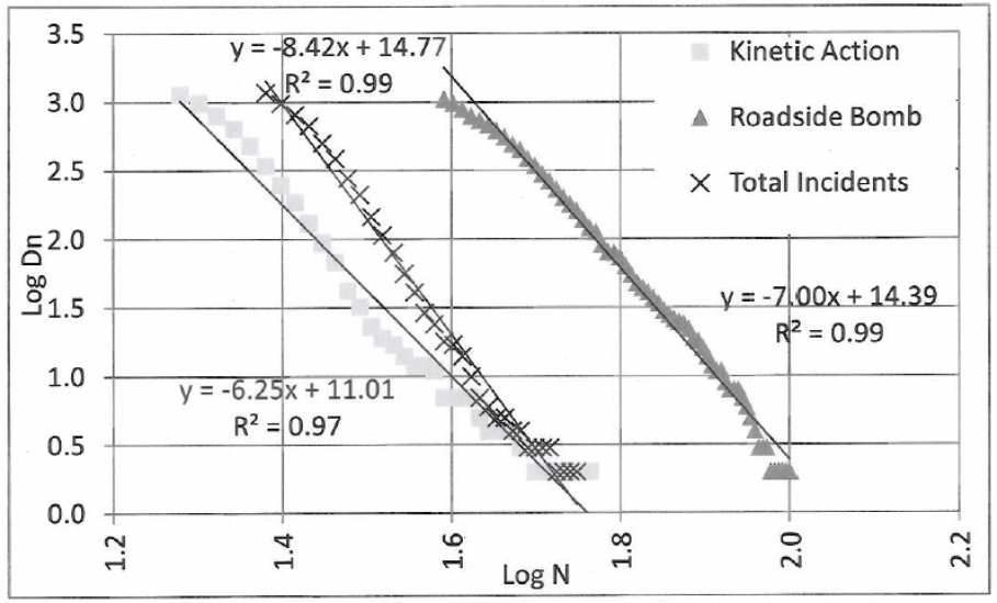
Figure 3 depicts the relationship between DN and N for low N; this relationship shows almost constant, near-zero occurrence of low counts, followed by a short transition period just before it reaches the median value.
Figure 4 depicts the relationship between DN and N for high N; defined as more than median renormalized Nmed. The log-log plot suggests power-law scaling between N and DN for both incident types, as well as for the total number of incidents. This is consistent with previous findings [1,3]; in these studies the scaling properties were interpreted as the violence levels being sustained in a near-critical or critical state.
The asymmetry in the distribution for low and high event counts relative to the expected behaviour (defined by monthly trends) suggests that only the positive deviations from monthly numbers constitute a fractal system, with possible interpretation of violence spike corresponding to explosive instabilities in meta-stable systems (as is discussed in Section “Violence as an Explosive Instability”). An obvious implication of a power-law distribution is the finite probability of extreme events. In other words, it is possible to have the number of daily incidents far above the median. The negative deviations appear to be of different nature and driven by different dynamics independent of the dynamics for large daily counts; the implications of this fact are discussed later.
Because of the change in global trends connected with the US troop surge in 2010–11 (Figure 1, arrested growth despite more contact opportunities), the authors looked at the scaling properties of daily incident counts before and after the surge (using 1 Jan 2010 as a pivot point). Somewhat surprisingly, there was almost no change in scaling properties, even the change in scaling coefficients was less than 10%. And, as will be mentioned in the next section, the same conclusion was arrived at for the persistence. This leads to a conclusion that while the global characteristics of the conflict changed, the critical nature of the conflict remained unchanged.
Method of detrended fluctuations
We now describe the methodology to examine persistence, viz. a measure of how future data are affected by past data. A signal that displays fractional Brownian motion (fBm) is one that has a zero-mean, and can be expressed as [8] the stochastic integral:
(2)
where W is a white noise process defined on (–∞,∞). Here is known as the Hurst parameter. The Hurst exponent for the signal is its roughness averaged over many length scales. The covariance function is given by:
so that and . This means that for the special case H = 1/2, fBm reduces to the well-known random walk, or Brownian motion. Typically, fBm is non-stationary, and thus detection of the presence of memory is a delicate task.
Brownian motion is an example of a process with short-range correlations, whose effects quickly peter out with distance from the source. Long-range correlations in time-series, in other words data whose effects are clearly observed for extended periods of time, can be tested for in numerous ways. A general methodology is to estimate how a characteristic size of the fluctuations (fluctuation measure), denoted here by F scales with the size n of the time window considered. Specific methods, such as Hurst’s rescaled range analysis [9], power spectral analysis, structure function analysis [10], or detrended fluctuation analysis [11], all essentially calculate such a fluctuation measure, although the measure is different for each technique. Typically, , where α is the scaling exponent. For a time series that follows a fBm the relationships between the scaling exponents of the various methods are simple.
Here we employ a DFA to the combat data. Novel ideas from statistical physics led to the development of DFA [11]. The method is a modified root mean squared analysis of a random walk designed specifically to be able to deal with nonstationarities in nonlinear data, and is among the most robust of statistical techniques designed to detect long-range correlations in time series [12–14]. DFA has been shown to be robust to the presence of trends [15] and nonstationary time series [16,17].
Briefly, the methodology begins by removing the mean, , from the time series, B(t), and then integrating:
The new time-series is then divided into boxes of equal length, n. The trend, represented by a least-squares fit to the data, is removed from each box; the trend is typically a linear, quadratic, or cubic function. Box n has its abscissa denoted by. Next the trend is removed from the integrated time series, y(k), by subtracting the local trend, , in each box.
For a given box size n, the characteristic size of the fluctuations, denoted by F(n), is then calculated as the root mean squared deviation between y(k) and its trend in each box:
This calculation is performed over all time scales (box sizes). A power-law scaling between F(n) and n indicates the presence of scaling:
where the parameter α is a scaling exponent; given a fractional Brownian motion series, the scaling exponent α = H—the familiar Hurst exponent (that is, the probability that an increase or decrease at a given time step will persist to the next time step). If α = 0.5 the signal is white noise; α < 0.5 indicates antipersistence and α > 0.5 indicates a persistent time series.
Dfa results
Figure 5 shows the results for kinetic action incidents between 1 Jan 2007 and 30 Jun 2012. The solid straight line is the best-fit linear curve to the data, with a slope α = 0.71±0.02. The best-fit is only applied to the first 75 percent of the fluctuation data. This is needed since finite size effects cause a roll-off of the fluctuations at largest scales. Figure 6 shows the results for the same time period for roadside bombs. In this case, α = 0.79±0.02. This implies that there is something inherent to the respective violence categories that causes this difference in the statistics (in terms of α). This may be related to the possible cost associated with each of the two attacks and/or properties of targets
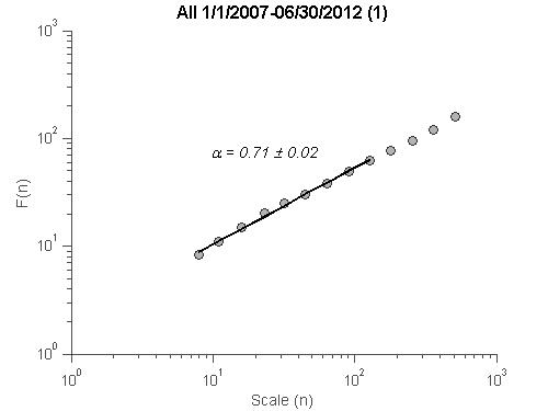
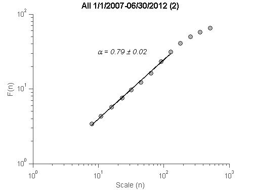
In both cases there is persistence with the exponent above 0.5. This means that a trend from one day to the next is most likely going to continue. If there were increases in violent incidents from one day to the next, the probability of the increase persisting on the next day is above 70% (α > 0.7). This result is generally consistent with the behavior expected for self-organized criticality, as demonstrated by Woodard et al. which showed that theoretically self-organized criticality exhibits persistence with α ~ 0.6 – 0.7 [19].
| Type of Attack | Kinetic | Roadside |
|---|---|---|
| All | 0.71±0.02 | 0.79±0.02 |
| Early | 0.70±0.02 | 0.80±0.02 |
| Late | 0.73±0.02 | 0.77±0.01 |
To address a possible effect of the US troop surge on the internal dynamics, the data were broken into two parts, before and after 1 Jan 2010. Table 1 summarizes these, and the previous results. In spite of surge of security forces, the essential statistical characteristics of the security incidents remain the same.
Incidents and casualties
To address fractal properties of the Afghanistan war from a different perspective, and to facilitate a direct comparison with the results in [2], the authors calculated scaling of casualties per incident using data between 2002 and 2012 (Figure 7). The result was a power-law scaling with the coefficient of –2.78. This is largely consistent with observations in [2]. However, the authors of this paper believe that reasons behind the scaling properties in the specific case of Afghanistan are somewhat different than the ones proposed by the authors of [2].
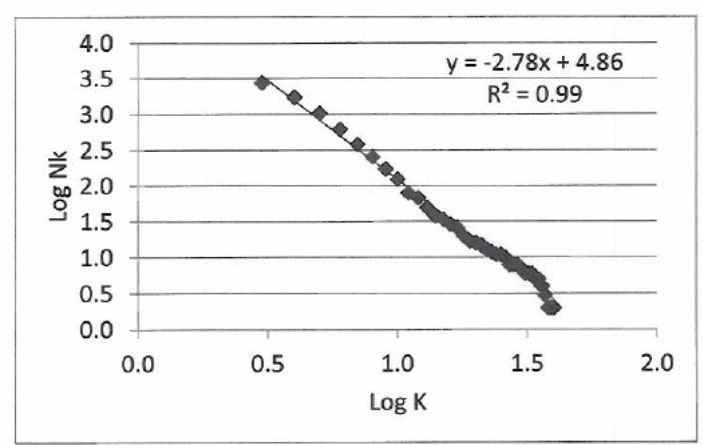
First of all, the assumptions made in [2] are not necessarily true for Afghanistan. The size of the security forces has not been constant, and most likely neither has the insurgent population. Between 2007 and 2010 there has been a steady increase in both Afghan and international forces; based on the proportional increase in the violence during this time frame, the insurgents have likely been able to counter this increase in security forces by increasing their own population and resources.
Furthermore, casualty numbers per incident are not necessarily related to the size of involved groups. There are important factors such as skills, training, terrain conditions, and other factors beyond the actors’ control that can play important roles in the outcome. There are also limits on how many casualties are theoretically possible for a particular incident. For instance, if insurgents attack a vehicle, the maximum number of casualties would be equal to the number of vehicle occupants irrespective of how many insurgents were involved. This limitation is specific to a large-scale insurgency targeting primarily military objectives, and it differs from a potential for casualties during terrorist attacks targeting civilians, such as the one used in the model [2].
Therefore a better model of violence would need to be able to account for dynamics specific for an insurgency, such as changes in force numbers and available resources, and the limitations on casualty numbers imposed by target characteristics rather than the attacking group’s size.
Violence as an explosive instability
As mentioned above, it is remarkable that the properties of the conflict in Afghanistan—a human interaction—are generally consistent with the dynamics of meta-stable physical systems, characterized by a time-dependent energy function (Hamiltonian) H(x,p,t) [18]. Such systems can be driven over time from stable to explosively unstable regimes in which any finite perturbation will lead to an avalanche-like release of energy that can be localized or can lead to a reconfiguration of an entire system [18]. The latter corresponds to a critical, the former to a sub-critical system [1,19].
The avalanche nature of such release renders responses often disproportional to actual triggers, and it also makes determining causality links dubious. This fact has potentially serious implications for interpretations of sudden shifts in incident numbers:
- Sudden, large changes in incident counts happening in response to minute changes in a system are a realistic possibility.
- The immediate cause of a change might be in principle intractable.
- Response can be delayed or happen in an unexpected way or at an unexpected location.
In terms of insurgency, the driving mechanism of increasing free energy may consider insurgent resources, supplies, command and control, and motivation. This increase would drive the system toward sudden redistribution of characteristic parameters (that is, spikes of violence above expected values). While the association of free energy with tangible and intangible resources seem obvious, the non-linear nature of the system implies that there is no direct causal relationship between a daily number of incidents and immediate shifts in resources. As long as the system remains stationary (that is, no global shift), the average amount of depleted resources will match the incoming supply. It is akin the behaviour of a sand pile. While the sand is added slowly, there will be avalanches of rolling sand; the size-frequency distribution of these avalanches will obey a power law, but it will be impossible to directly connect a particular load of sand to a particular avalanche.
On the other hand, the low daily counts (decreases from expected values) do not follow a power law. In terms of the Hamiltonian approach they would correspond to declines in energy redistribution, and thus would be connected to external removal of available energy (energy sinks). This would likely be connected with disruptions to the resources or motivation of the enemy (removing sand from the pile). Unlike the response to adding more resources, in this case the response would depend on the location of the sink. Using the analogy of the sand pile, if the sand is at first removed from one side and then additional sand is added at another side, there might be little to no response to avalanche scaling. But if the sand is added at the location of sink, losses need to be replaced before avalanches can be triggered.
What sets Afghanistan apart from general stationary systems is the presence of long-term trends driven by external factors such as security forces’ strength, or weather and climatic conditions. In the proposed model these trends can be considered as Hamiltonian modifiers.
There is a body of work suggesting that a wide variety of self-organized critical systems fall into a universality class [20–22] characterized by common scaling properties. Previous research also found that for non-conservative systems (that is, systems with a time-dependent Hamiltonian) the power-law behaviour breaks down once a systems’ characteristic scale is reached [20]. The latter was indeed observed for the casualty/incident distributions, when the breakdown occurs for approximately 30 casualties per incident (this maximum scale is dependent on the type of operations and/or units involved). This further strengthens the arguments in favour of the Hamiltonian model of insurgency.
Summary and conclusions
The present paper revisited analyses of fractal properties of the conflict in Afghanistan using significantly larger data set than the original studies [1,3]. This study confirms in part the general findings of these earlier studies. The insurgency in Afghanistan behaves indeed as a critical system, but strictly speaking it may not be entirely self-organized. The size-frequency distribution for positive variations from expected behaviour (based on monthly averages) indeed obeys a power law; on the other hand negative variations do not adhere to such scaling. This is likely stemming from different drivers behind the two types of variations.
Using DFA we confirmed that the daily incident counts are indeed persistent, with the Hurst coefficient around 0.7 which is typical for self-organized criticality [19]. This is possibly connected with the dynamics of the positive variations.
There was no shift in either scaling properties or persistence corresponding to the surge in 2010. This suggests that while the surge changed gross global properties of the system (availability of resources, will, and capacity to absorb incidents) reflected by actual trends, the local properties (the complex nature of the conflict) remained largely unchanged. This points to a possibility of a universal character of large scale counter-insurgencies like the one in Afghanistan. This is consistent with the fact that most insurgencies would be characterized by similar types of violence (such as ambushes, whether kinetic or using bombs; terrorist attacks; attacks on installations; and assassinations). They would be also characterized by the insurgent avoidance of direct force-on-force engagements involving large units as this would usually expose them to far superior firepower. Existence of such a universality class for conflicts might potentially enable modeling of such conflicts, with direct application in logistics and force planning.
This paper argues that the previous stationary model explaining power-law scaling in terms of aggregating or splintering terrorist groups is inadequate for the conflict in Afghanistan, since some of the fundamental assumptions of the model do not hold for this conflict. While the stationary model may hold for traditional terrorist violence, it breaks down for non-stationary and large scale insurgencies such as the conflict in Afghanistan. An alternative model based on the explosively unstable non-conservative systems is proposed. Such model in principle enables incorporating external factors such as increase in security forces or counter-insurgency operations. The model would also allow for the asymmetry in the behaviour of high and low incident counts, and it is consistent with the existence of characteristic scales.
References
[1] P. Dobias, “Self-Organized Criticality in Asymmetric Warfare”, Fractals, Vol. 17, No. 1, Mar 2009, pp. 91–97.
[2] J.C. Bohorquez, S. Gourley, A.R. Dixon, M. Spagat, and N.F. Johnson, “Common Ecology Quantifies Human Insurgency”, Nature, Vol 462, 17 Dec 2009, pp. 911–914.
[3] P. Dobias and K.B. Sprague, “Intermittency of Casualties in Asymmetric Warfare”, Journal of Battlefield Technology, Vol. 12, No. 1, 2009, pp. 19–25.
[4] J.A. Wanliss, P. Dobias, and K. Sprague, “Persistence in Significant Activities in Afghanistan”, Journal of Battlefield Technology, Vol. 13, No. 3, 2010, pp. 25–29.
[5] International Security Assistance Force, Monthly Violence Trends, published monthly at www.isaf.nato.int.
[6] E. Gons, J. Schroden, R. McAlinden, M. Gaul, and B. VanPoppel, “Challenges of Measuring Progress in Afghanistan Using Violence Trends: The Effects of Aggregation, Military Operations, Seasonality, Weather, and Other Causal Factors”, Defence & Security Analysis, Vol. 28, No. 2, 2012, pp. 100–113.
[7] T. Hill and P. Lewicki, Statistics: Methods and Applications, StatSoft, Tulsa, OK, 2007; (Electronic version: StatSoft, Inc.. Electronic Statistics Textbook. Tulsa, OK: StatSoft, 2012. WEB: http://www.statsoft.com/textbook/).
[8] B.B. Mandelbrot and J.W. Van Ness, “Fractional Brownian Motions, Fractional Noises and Applications”, SIAM Review, Vol. 10, No. 4, 1968, pp. 422–437.
[9] H.E. Hurst, “The Long Term Storage Capacity of Reservoirs”, Transactions of American Society of Civil Engineering, Vol. 116, 1951, pp. 770–799.
[10] V.I. Abramenko, V.B. Yurchyshyn, H. Wang, T.J. Spirock, and P.R. Goode, “Scaling Behaviour of Structure Functions of the Longitudinal Magnetic Field in Active Regions on the Sun”, Astrophysical Journal, Vol. 577, No. 1, 2002, pp. 487–495.
[11] C.-K. Peng, S. Havlin, H.E. Stanley, and A.L. Goldberger, “Quantification of Scaling Exponents and Crossover Phenomena in Nonstationary Heartbeat Timeseries”, Chaos, Vol. 5, No. 1, 1995, pp. 82–87.
[12] M.S. Taqqu, V. Teverovsky, and W. Willinger, “Estimators for Long-range Dependence: An Empirical Study”, Fractals, Vol. 3, No. 4, 1996, pp. 785–798.
[13] H.J. Blok, On the Nature of the Stock Market: Simulations and Experiments, PhD thesis, University of British Columbia, Canada, 2000.
[14] M.J. Cannon, D.B. Percival, D.C. Caccia, G.M. Raymond, and J.B. Bassingthwaighte, “Evaluating Scaled Windowed Variance Methods for Estimating the Hurst Coefficient of Time Series”, Physica A, Vol. 241, No. 3, 1997, pp. 606–626.
[15] K.P. Hu, Ch. Ivanov, Z. Chen, P. Carpena, and H.E. Stanley, “Effect of Trends on Detrended Fluctuation Analysis”, Physical Review E, Vol. 64, No. 1, 2001, 011114.
[16] J.W. Kantelhardt, S.A. Zschiegner, E. Koscielny-Bunde, S. Havlin, A. Bunde, and H.E. Stanley, “Multifractal Detrended Fluctuation Analysis of Nonstationary Time Series”, Physica A, Vol. 316, No. 1, 2002, pp. 87–114.
[17] Z. Chen, P.Ch. Ivanov, K. Hu, and H.E. Stanley, “Effect of Nonstationarities on Detrended Fluctuation Analysis”, Physical Review E, Vol. 65, 2002, pp. 041107.
[18] P. Dobias, J.A. Wanliss, and J.C. Samson, “Nonlinear Stability of the Near-Earth Plasma Sheet During Substorms: 9 February 1995 Event”, Canadian Journal of Physics, Vol. 84, 2006, pp. 1029–1047.
[19] R. Woodard, D.E. Newman, R. Sanchez, and B.A. Carreras, “Persistent Dynamic Correlations in Self-Organized Critical Systems Away From Their Critical Point”, Physica A, Vol. 373, 2007, pp. 215–230.
[20] K. Christensen, Self-Organization in Model of Sandpiles, Earthquakes, and Flashing Fireflies, Thesis, Institute of Physics and Astronomy, University of Aarhus, Denmark, 2002.
[21] A. Chessa, H.E. Stanley, A. Vespignani, and S. Zapperi, “Universality in Sandpiles”, Physical Review E, Vol. 59, No. 1, 1999, pp. R12–R15.
[22] A. Vespignani, S. Zapperi, and L. Pietronero, “Renormalization Approach to the Self-organized Critical-behavior of Sandpile Models”, Physical Review E, Vol. 51, No. 3, 1995, pp. 1711–1724.