Forecasting Conflict Intensity: Afghanistan

Introduction

Conflict intensity data, which includes improvised explosive device (IED) strikes, small arms fire, fatalities, and other violent incidents in the Afghanistan operational theatre, with daily temporal resolution from 1 January 2005 to 30 June 2011, has been unclassified and forms the time series under consideration (see Figure 1). The source data originated from the Combined Information Data Network Exchange (CIDNE, US DoD). The time series is characterized by a smoothly varying mean level, enveloped by stochastic fluctuations. The mean level displays both seasonal variations and global upward growth, while the fluctuations scale with the mean level.

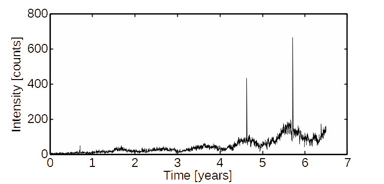
In addition to the regular pattern exhibited in day-to-day conflict levels, three large and anomalous spikes occur in the vicinity of election days. This election day violence appears to be cleanly decoupled from the day-to-day violence, allowing the day-to-day and election day violence to be decomposed and independently analyzed. Due to similar (identical within error) long-term growth of the two, and the occurrence of elections near the seasonal peak in day-to-day violence, it can be conjectured that ≈1/6 to 1/5 of anti-coalition “force potential” is projected on a given day. The large, but bounded, latent force estimate allows meaningful scenarios to be considered. This paper includes a discussion on how the conjecture may enable total anti-coalition personnel to be estimated.

Day-to-day conflict levels are decomposed into mean levels, via smoothing, and stochastic residual. Gross forecasting of the trend is enabled as the mean conflict level exhibits long-term growth which approximately follows a parametric (exponential) form. However, forecasting is difficult due to sizeable seasonable variation overlaying the basic exponential growth – which is cyclic, but without a sharp, precise, period – and limited data. A “seasonal template” approach to facilitate forecasting is outlined.

In regards to the noisy fluctuations, the stochastic residual can be cast into a stationary form as the fluctuation magnitude is related to the mean level, allowing surrogate (synthetic) data to be generated and the stochastic fluctuations which envelope the mean to be forecasted.

Given the degree of change in Afghanistan over the period examined, the varying levels and forms of international intervention, and the complexities surrounding how influential decision makers arrive at their courses of action, it may be thought that little value can be gained from analyzing violence from a “signals” perspective. As is demonstrated in this work, the consistency of the pattern of violence contravenes the naïve expectation that the dynamical system is essentially too complex to make plausible projections against. Apparently, for violence in Afghanistan it is not, and analyzing such “signals” for valuable insights into conflicts has become commonplace and is supported by an ever growing body of evidence (see, for example [1–6]).

Network inspired model

A simple network inspired model is taken as a working hypothesis – where participants’ access to the theatre of combat (“the network”) is based on their availability and intent, and conflicts arise based on random happenstance, skill level, ongoing campaigns and operations, and other factors which are hard to meaningfully identify and capture within a well calibrated model. As such, general conflict intensity levels are regulated by participants’ “access to the network” (intent and means to engage in the operational theatre), with a large (quite possibly correlated) stochastic component. Further, such a model suggests that fluctuations will scale with the overall conflict level, as fluctuations arise from the intersection of intent, opportunity, and happenstance, and one would expect a number of timescales to exist (see [7] for an excellent exposition on network scaling properties). These basic features motivate using a smoothing function to determine the general intensity level about which observed conflict will fluctuate.

As noted, it was empirically found that the time series can be decomposed into these two elements: a smoothly varying trend which captures longer-term dynamics, together with rapid, correlated, stochastic fluctuations (the residual) around that trend. Power-law scaling, perhaps the simplest model, is considered to describe the fluctuations. It is found that this hypothesis allows the residual to be cast into stationary form (e.g., the model is a reasonable approximation), opening up the ability to analyze and manipulate the fluctuations—including the ability to forecast future fluctuation magnitudes.

Mean conflict levels

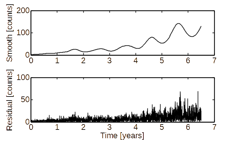
Loess filtering [8] with a 2nd order (quadratic) polynomial was performed using the closest year of data, resulting in a smoothed curve describing the mean conflict intensity level. The residual around the mean level is taken to describe the rapid timescale stochastic fluctuations. To remove the election day violence spikes, the peaks were excised (as described below).

Decomposing election day and day-to-day violence

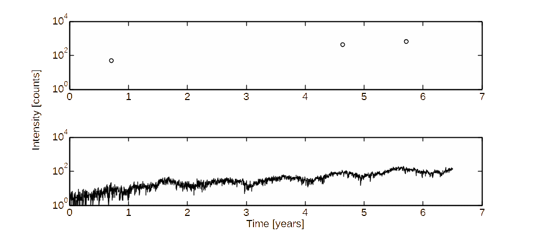
The data set was decomposed into two subsets analyzed separately—the election day violence spikes, manually selected, and a day-to-day violence time series (Figure 2). Removal of election day violence induces gaps in the time series. To reduce the possibility of pre- and post-election day dynamics from affecting the day-to-day series, the gaps are widened by three days on either side and the intervals filled via artificially created synthetic data generated from an iterative imputation procedure (see “Forecasting: Stochastic Component and Decomposition”, below, for details).

Estimates of long-term growth

Performing a linear fit to the logarithmically scaled election-day violence (for example, exponential fitting) results in an exponential growth rate of rate λ = (145.2 ± 7.6) × 10^–5 /day. Yearly binning of day-to-day violence demonstrates an exponential growth rate of λ = (144.7 ± 15.5) × 10^–5 /day. These two violence types exhibit identical, within error, growth rates.

Coalition military fatalities [9] in Afghanistan also exhibited approximate exponential growth over the same time period, with a growth rate of λ = (91.6 ± 0.3) × 10^–5 /day (estimated using yearly totals, from 2005 to 2010). This growth rate is comparable to that exhibited by our aggregate violence measure, indicating that our more inclusive measure can provide insight on a primary concern: expected fatalities, and suggests expected injuries may likewise be projected, but at the cost of incorporating additional information (for example, force strength and exposure to violence).

Forecasting

It is clear that one cannot hope to predict a complex and evolving situation with high fidelity: there simply are too many uncertainties involved. It has long been recognized that uncertainties (“unknowables”) are fundamentally different than risk (which follows a distribution that can be calibrated against observations) [10]: essentially any system driven by human action is inherently unpredictable. For example, one cannot accurately predict the price of oil or long horizons [11] even though (or perhaps, because) the use of oil is a fundamental driver of the modern world. Despite these clear caveats, forecasting is of interest and value: if the effectively unknowable forcing mechanisms slowly change, then short-range forecasts are viable, and given plausible models one can gain some insight into likely outcomes.

Forecasting: stochastic component and decomposition

The stochastic component is cast into a stationary form and forecast via Iterative Amplitude Adjusted Fourier Transform (IAAFT) generated surrogate time series [12].

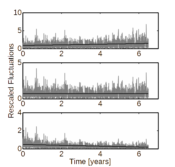
It is empirically found that the magnitude of fluctuations scales with the mean intensity (see Figure 3, compare the residual magnitude with the smooth (mean level) and note that fluctuation magnitude scales with the local mean). Testing a simple power-law scaling hypothesis suggests that fluctuations δ follow such a scaling:

$\left|\delta \right|\propto I^{\alpha }$ (1)

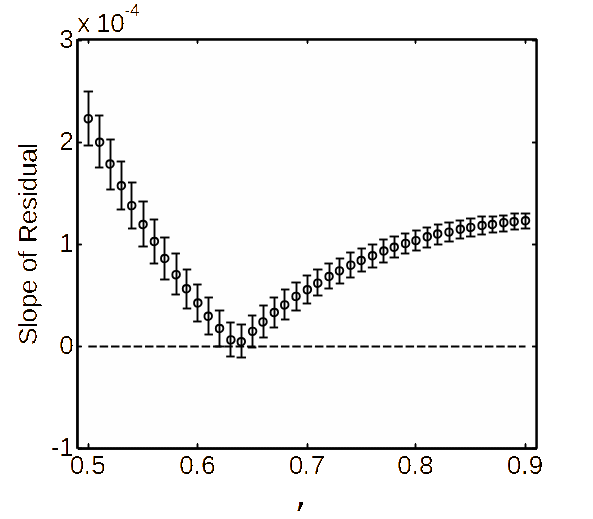
where I is local intensity (smoothed counts as per Figure 3 (top)) and α is the power-law scaling exponent. It is found that α = 0.63 ± 0.01 is the best estimate (see Figures 4 and 5). In order to estimate the exponent, the fluctuations are rescaled for a given α and the rescaling tested for stationary traits. A best linear fit was performed on the scaled fluctuations, probing for the constant level (zero slope) characteristic of stationarity. The error is estimated by finding all slopes that are zero within fitting error.

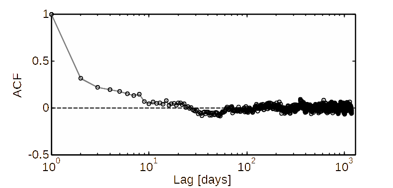
The autocorrelation function (ACF) of the stationary (rescaled) fluctuations displays correlated temporal dynamics, with a characteristic time scale of roughly one week (three e-foldings in ≈10 days), see Figure 6.

By casting the fluctuations into a stationary space, a surrogate time series can be constructed; here IAAFT is used [12]. IAAFT is a latent Gaussian model that exactly reproduces the distribution and approximates the spectrum of a time series, essentially reshuffling the data under the constraint that it must match a given ACF.

Here an iterative enveloping algorithm is used—as noted previously large outliers corresponding to election-day violence and, as a result, the distribution and ACF will be strongly affected. To mitigate such effects, data in the immediate vicinity of election days are excised and the intervals refilled with randomly drawn data (recall that the necessary manipulations are being performed in rescaled residual space, which is nominally “flat”). The ACF is then found, IAAFT performed, and the IAAFT surrogate is used to fill in the gaps. The procedure is then repeated, incrementally eliminating the effect of removing the outliers and nearby data. There is one additional subtlety to this procedure: the surrogate data sequence filling in the gaps must match the data at the boundaries, and so subsequences are found that best satisfy this constraint. In such a manner outliers are removed, imputing and infilling removed data with distributional and spectral characteristics matching the day-to-day violence outside of the election day regions, thereby decomposing the time series into two sets: one corresponding to election-day violence and the other to day-to-day violence.

Forecasting: mean level

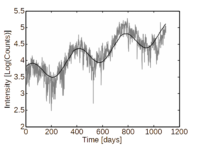
Despite the clear seasonality of the data, the observed variation in seasonal period leads to significant year-to-year scaling of seasonal variation (in the most recent four years the cycle was off a standard year by –1, 3, –22, and 5 days, respectively), preventing a straightforward extrapolation of the violence cycle. See Figure 7 where a linear fitting and forecast is performed on the latest 3 (logarithmically transformed) years. While overall good performance is obtained, the recorded data wanders around a strict yearly period and in particular, the last months of data in the cycle (that is, most salient data for forecasting) happen to not closely follow patterns observed in the average cycle. Thus, while on average a linear model provides reasonable forecasts, the sizeable variation in the year-to-year seasonal period can lead to sizeable discrepancies between the fit and the observations. Experiments on synthetic data (not shown) indicate that a diffusing phase in a pure sinusoid—characterizing a perfectly periodic cycle with induced phase error—leads to similar behavior, with good average performance and occasional large (unsystematic) deviation.

Due to variation in yearly cycles, medium-term forecasts will be uncertain, making, for example, Holt-Winters predictions (possibly much) less accurate than in-sample errors would tend to indicate. In order to address this variable periodicity, and the clear discrepancy between the average (expected) and observed records for the latest data, a “seasonal template” is constructed (described in more detail below), where cycles are scaled and averaged together to define the reference template. This template can be fitted to the most recent partial cycle, allowing medium-term forecasting throughout the cycle.

Forecasting

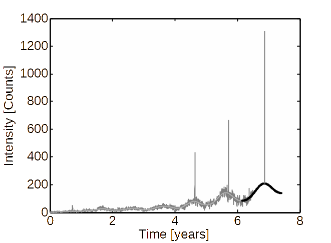
The template (Figure 8, inset) is scaled to best fit the latest partial data, allowing medium range forecasting (Figure 8). The counterfactual case of an election occurring in 2011 demonstrates that, if underlying dynamics remain largely unchanged, a doubling of violence over that of 2010 is expected (see below for further discussion).

Surrogate data can be used to create many possible paths, indicating the expected range in violence and visually underscoring the noisiness of the dynamics; see Figure 9 where 10 possible future paths are plotted (9 in light grey, to demonstrate the envelope of expected fluctuations around the mean, and 1 in dark grey to emphasize the detail of one specific, possible future). It can be seen that violence ranges rather dramatically around the mean, underscoring the importance of examining both the smoothed values and the ranges in order to set realistic bounds on expectations.

Discussion

Model used

Smoothing with local regression methods, such as Loess, performs similarly to other nonparametric approaches and has the advantage of automatically correcting for boundary bias (see page 193 of [13] for a brief discussion). Loess is a good choice for smoothing in this case, since the most recent and salient data is, by definition, near a boundary (data cutoff) where induced bias will be most detrimental (for both “nowcasting” [14] and forecasting).

As discussed, the mean cannot be forecasted with classic approaches that account for seasonality, such as Holt-Winters [15], as the seasonal periods exhibit sizeable variation. This variation in cycle motivates the template approach, where accuracy within a given cycle (short/medium-term prediction) is sought, unfortunately at the cost of long time horizon predictability.

Casting the fluctuations into a stationary form decomposes the data into election day violence and day-to-day violence, enabling forecasting of future fluctuations, as in Figure 9. Note the time series is fairly short, and the absolute number of counts is rather small near the start of the time series (increasing relative error), a concern in estimating the best scaling parameter. A sensitivity analysis supports the 0.63 ± 0.01 best value on the whole data set, where the time series is shortened to 2/3rds the length and rescaling is performed on the first and last two thirds, resulting in scaling parameter estimates of 0.57 ± 0.03 and 0.58 ± 0.05.

In excluding the outlying election day spikes from day-to-day violence, the procedure—with surrogate imputed substitution near the spikes—is only asymptotically correct, while only the first two iterations are performed here. Little difference (within random noise) in the autocorrelation and a smooth curve is found to occur beyond the first iteration, indicating quick convergence.

In defining and excluding election day violence, visual inspection was used to define the period to exclude (three days on each side). Selection of a larger period (10 days on each side) results in identical (within error) estimates of the exponential characteristic times of the trends with no observed systematic change in the obtained smooth curve, indicating that the excluded period chosen is sufficient, and lending support to the notion that election day violence is largely decoupled from the underlying day-to-day violence.

Errors

In fitting exponential trends standard errors are reported, the standard deviation is used in all other cases.

Underlying causes?

With sparse and noisy data great care is required to avoid identifying patterns and change points (where driving dynamics change) that are not well supported by the data.

The data itself is an aggregate measure, which may be affected by non-uniform reporting. It is thought sigact (significant actions) reports may have up to a ≈10% bias towards underreporting [6]—with the precise bias possibly contingent on operational issues (that is, changing over time), introducing additional uncertainty.

The smoothly varying trend displays seasonal variation, a well-known feature that has been attributed to the agricultural basis of Afghanistan society [16]. However, a multitude of factors are involved with the changing seasons. While harvest may be important, the decreased vegetative cover in winter months makes both IED placement and ambush more difficult, hardened and dried soil makes IED emplacement less effective, fresh snowfall in mountainous regions precludes undetected travel making IED emplacement or ambush difficult [17].

While a direct linkage to coalition troop levels has been identified elsewhere, as in [16] where regression analysis is used, it should be noted that both violence and troop levels are monotonically increasing (over long time horizons), which ensures a correlation. However the trooping levels display approximate linear growth until roughly July 2009 (see Figure 3, in [16]), at which point they exhibit a sizeable increase and qualitative change from linear to concave down growth. Note that there is no unambiguous corresponding change point in the recorded violence data (see Figure 2, both here and in [16]). The absence of a corresponding qualitative change in the violence data is more supportive of a relatively small number of insurgents consistently enacting their agenda, versus a direct reactionary opposition to trooping levels, and cautions against linking violence levels to the coalition force size (both for interpretation, and in modelling – as this may induce misspecification in the model, resulting in worsening predictive performance). Note the distinction between tracking overall violence levels, as is done here, vs. tracking coalition casualties, which is often reported on and forms a subset of the violence data.

Numerous possible patterns and change points exist—Pakistan ceding control of FATA’s North Waziristan region to tribal chiefs associated to the Taliban [18] in September 2006 (the data, see Figure 2, weakly supports this changing of the underlying dynamics, however, note the absolute number of incidents is quite low making it difficult to discern any linkage), the increase in troops levels near the end of 2009 (see discussion above), Ramadan ([16] found no significant correlation), poppy harvest (both [16] and [6] identify a significant correlation), and the drawdown of US trooping levels starting July 2011 [19] (just off the end of the available data set) are some important possible influences on violence. There are essentially unlimited possible, and even plausible, hypotheses, and if one searches through them one is ensured to find many “supported” by the data, just by idiosyncrasy in the noise happening to align with the purported pattern. It is likely most fruitful to focus on highly pronounced characteristics of the data and keep in mind that sizeable fluctuations and timescales exist: it is both difficult to accurately discern subtle patterns in the sizeable noise (both real, and possible reportage induced) and such patterns are of less concrete concern, as they will be subtle/weaker in effect. Here the most pronounced characteristics found are 1) an approximately exponential trend for both day-to-day and election day violence; 2) the fluctuation magnitude appears to (power-law) scale with the local average violence intensity; and 3) sizeable seasonality exists.

Elections

Elections and the violence associated with them occur near the seasonal peaks, and both election day and day-to-day violence display identical growth. This suggests that near maximal force projection occurs during election campaigns and that ≈1/6 to 1/5 (more precisely, 5.65 ± 0.97) of available force is projected day-to-day. The reasoning behind this hypothesis is essentially Occams razor [20]. As the Taliban issue a strong edict against the elections [21], the events provided a strong rallying point. The strong pull combined with the fact that the elections coincide near the seasonal peaks of violence (for example, when the pool of anti-coalition participants are most available for combat) suggests that near universal participation of anti-coalition forces is plausible. As both day-to-day violence and election day violence grow at the same rate (within error), the simplest explanation is that the ratio of participants in both of these modes is constant. If election day violence marks peak, near universal, participation, this indicates ≈1/6 to 1/5 of available anti-coalition forces operate day-to-day.

The tenable finding that ≈1/6 to 1/5 of anti-coalition forces operate day-to-day (during peak availability) and near universal participation occurs at election days provides valuable insight on various worsening-case scenarios, and in combination with additional information (for example, estimated number of anti-coalition troops on a given day) may provide useful estimates on the total number of radicalized forces.

In Figure 8 the (counter factual) scenario of an election being held at the peak of the predicted cycle in 2011 is shown, visually demonstrating the dramatic effects of the (exponential) increase in likely violence. It is important to note that if the ground situation does not change, and the next election comes near the seasonal peak in day-to-day violence as historically done, this prediction of ≈ 1300 counts of violence represents a near doubling in election day violence yet underestimates expected violence. The next election is not solidly set but is provisionally slated for 2014. This horizon is far enough in the future to induce significant uncertainty in the appropriateness of precise predictions based on the limited data, however a doubling in violence over that experienced in 2010 seems likely, and if trends continue, violence will be nearly an order of magnitude larger for a 2014 election. Great care must be taken as even small error in the fitting will strongly affect forecasts, and such error is well expected for such distant time horizons (relative to available data). Furthermore, this projection assumes no change in underlying conditions while the drawdown of coalition forces is underway and will be collocated with the election [19]. Nevertheless, this possible, dramatic, increase in violence is suggested by the available data.

In considering election day violence forecasting, it should be emphasized that all prior election days occurred near the peak of day-to-day violence cycles. If a future election is held off of the peak, it is unclear whether an exponential extrapolation will provide accurate expectations as such a forecast may overestimate violence. It may be more appropriate to forecast a ≈ 6X expected daily violence level, and use the exponential forecast as an expected worse case level.

Forecasting

It should be emphasized that exponential growth cannot be sustained, given limited resources (i.e., number of available Afghan, or foreign, persons to be recruited). When resources become constrained one typically observes an “s-curve” [22] where initial exponential growth slows, rolls over, and plateaus. The data does not reveal the presence of such a roll over. A negative implication is that growth in violence may be quite unconstrained, while a positive implication is only a small fraction of Afghanistan society is involved and violent actors are not widespread, which suggests a strong role for the “Hearts and Minds” doctrine [23].

The demographic growth in Afghanistan is roughly exponential, providing one possible driver for the increase in violence. However, the effect is over a magnitude too small to account for the increase in observed violence, as the growth rate in the fighting age bracket of Afghanistan is ≈ (5-10) x10^-5 /day, with the precise value depending on various assumptions made regarding the age mixture of insurgents. This suggests that while changing demographic profile alone can account for some of the violent increase, demographics are quite insufficient to explain the magnitude of the observed increase.

The general exponential trend allows quick, rough, estimates to be made under the assumption of persistent dynamics. In particular, the mean and bounds (seasonal peak/troughs) can be readily made. Further, the power-law relationship between fluctuations and mean levels also enables day-to-day variation to be estimated. While long-term forecasting is clearly on uncertain ground, as the factors underlying the observations are bound to change, a simple linear (of transformed data) model, such as in Figure 7, appears quite reasonable for forming expectations. For the current upcoming months and year, the template model provides a fairly compelling means of forming expectations. The model exchanges long-term ability to predict for higher fidelity in the upcoming cycle. While various means of bridging these two horizons may exist, there is both little evidence to constrain models and (relatively) limited gain to be had. The violence data examined exhibits a fairly consistent pattern belying the assumption that rich dynamic systems are too complex to make plausible projections against. The underlying drivers have undergone sizeable changes over the period examined, yet predictability remains. One possible explanation is that in such high stake environments “all out” efforts drive some system parameters to their extreme boundaries. As such, the proximate and specific actions taken may be highly idiosyncratic, novel, and unpredictable, yet lead to relatively stable results.

Conclusions

In summary, smoothing enables long-term trends in the aggregate conflict data to be captured and a stochastic envelope of fluctuations defined. These components can be independently forecasted and combined to provide the expected conflict level and stochastic envelope. An approximately exponential trending growth is found, exhibiting significant seasonal variation, and nominal power-law scaling of the fluctuation on the mean conflict level was also determined. Surprisingly, election day conflict intensity displayed identical (within error) growth as day-to-day violence, suggesting that day-to-day violence is directly proportional to number of anti-coalition operatives and that election day campaigns capture near universal participation of the group while day-to-day violence during the seasonal peaks involve approximately 1/5 to 1/6 of total anti-coalition participants. Notably, it is found that – if the dynamics of the data set analyzed persist – the next election, slated for 2014, will experience more than twice the violence of the 2010 elections, with a possible, and extraordinary, 10-fold increase.

Acknowledgements

The authors would like to thank Peter Dobias of Defence Research and Development Canada (DRDC) for providing the data set used, and Phil Eles of DRDC for informative discussions. RMB is supported by a Natural Sciences and Engineering Research Council of Canada Visiting Fellowship. This work was completed under the DRDC CORA Technology Investment Fund Exploring Critical Behaviour in Warfare (2009-2012).

References

Authors

R.M. Bryce obtained his PhD in Condensed Matter Physics in 2010 (University of Alberta) and is currently an NSERC Visiting Fellow at DRDC, focusing on data analytics/operational research. He can be contacted at Robert.Bryce@drdc-rddc.gc.ca.

Kevin Sprague obtained his PhD in Theoretical Physics and Applied Mathematics at the University of Western Ontario and now works for the DRDC Centre for Operational Research and Analysis.

References

[1] J.C. Bohoroquez, S. Gourley, A.R. Dixon, M. Spagat, N.F. Johnson, “Common Ecology Quantifies Human Insurgency”, Nature, Vol. 462, No. 17, pp. 911–914, 2009.
[2] J. Wanliss, K. Sprague, P. Dobias, “Detrended Fluctuation Analysis of Combat in Afghanistan”, Journal of Battlefield Technology, 13(3), pp. 25–29, Nov 2010.
[3] K. Sprague, P. Dobias, R. Bryce, “Critical Behaviour in Patterns of Violence in Afghanistan”, Journal of Battlefield Technology, 14(1), pp. 17–24, Mar 2011.
[4] K. Sprague, P. Dobias, “Intermittency of Casualties in Asymmetric Warfare”, Journal of Battlefield Technology, 12(1), pp. 19–25, Mar 2009.
[5] A. Clauset, C.R. Shalizi, M.E.J. Newman, “Power-law Distributions in Empirical Data”, SIAM Review, Vol. 51, pp. 661–703, 2009.
[6] P. Dobias, P.T. Eles, J. Schroden, and J. Wanliss, “Quantitative Assessment in Support of Military Intelligence: Predictive Analysis and Risk Assessment in the Current Security Environment”, Proceedings from the 28th International Symposium on Military Operational Research, 2011, Hampshire, UK
[7] W.E. Leland, M.S. Taqqu, W. Willinger, and D.V. Wilson, “On the Self-Similar Nature of Ethernet Traffic (Extended Version)”, IEEE/ACM Transactions on Networking, 2(1), pp. 1–15, 1994.
[8] W. S. Cleveland and S. J. Devlin, “Locally-Weighted Fitting: An Approach to Fitting Analysis by Local Fitting”, Journal of the American Statistical Association, 83, pp. 596–610, 1988.
[9] See www.icasualties.org.
[10] F.H. Knight, Risk, Uncertainty, and Profit. Hart, Schaffner & Marx; Houghton Mifflin Co., 1921.
[11] S. Makridakisa, R.M. Hogarth and A. Gabac, “Forecasting and Uncertainty in the Economic and Business World”, International Journal of Forecasting, 25(4), pp. 749–812, 2009.
[12] T. Schreiber and A. Schmitz, “Improved Surrogate Data for Nonlinearity Tests”, Physical Review Letters, 77, pp. 635–638, 1996.
[13] L. Wasserman, All of Nonparametric Statistics, Springer, 2010.
[14] H. Choi and H. Varian, “Predicting the Present with Google Trends”, Economic Record, 88(s1), pp. 2–9, 2012.
[15] P.R. Winters, “Forecasting Sales by Exponentially Weighed Moving Averages”, Management Science, 6(3), pp. 324–342, 1960.
[16] E. Gons, J. Schroden, R. McAlinden, M. Gaul, and B. Van Poppel, “Challenges of Measuring Progress in Afghanistan Using Violence Trends: The Effects of Aggregation, Military Operations, Seasonality, Weather, and Other Causal Factors”, Defense & Security Analysis, 28(2), pp. 100–113, 2012.
[17] P. Eles (DRDC CORA), personal communication, July 2012.
[18] “Government, Militants ‘Ink’ NWA Peace Pact”, The Nation (Pakistan), September 2, 2006.
[19] D. Reichmann, “US Afghan Drawdown Halfway Done”, AP News, 22 July 2012.
[20] D.J.C. MacKay Information Theory, Inference, and Learning Algorithms, Cambridge University Press, Cambridge, 2003.
[21] S. Yousafzai, “An Inviting Target”, Newsweek, Aug 17, 2009.
[22] N. Boccara, Modeling Complex Systems, Springer, 2010.
[23] Headquarters, Department of the Army, Army Counterinsurgency Field Manual FM-3.24, 2006.