Feature-Based Target Recognition In Infrared Images For Future Unmanned Aerial Vehicles

Feature-based target recognition in infrared images for future unmanned aerial vehicles

Introduction

Worldwide interest in unmanned aerial vehicles (UAVs) has been increasing in recent years. Market research [1] suggests that UAV markets are forecast to reach $7 billion dollars worldwide by 2017. Primarily, there has been impressive growth in the demand for UAVs by the United States military since 2001 [2], driven by their successful contributions to campaigns in Afghanistan and Iraq [3], although interest in UAVs in Asia [4] and Europe [5] is also growing.

Consequently, research into new technologies to advance UAV systems is currently an important field [6]. The US Navy is making large investments in a number of UAV programs [2], and both the US Army [7] and Air Force [8] have unveiled roadmaps for future UAV development in the coming years. In the long-term, it is hoped that unmanned aircraft will be able to engage targets with some level of autonomy. To do so would require on-board processing such as automatic or aided target recognition [7].

Some manufacturers of UAVs have already claimed that their systems are capable of autonomous operation [6]. Taranis, for example, is an Unmanned Combat Aircraft System advanced technology demonstrator from BAE Systems, which is claimed to be able to “autonomously control the aircraft to taxi, take off and navigate its way to a search area while reacting to any threats” [9]. In order to react to threats, it is likely that some form of target identification must be present.

This evidence suggests that automatic target recognition (ATR) and identification for future UAVs is an emerging research area worthy of investigation. This paper thus considers the task of object recognition for the possible introduction of target discrimination capabilities in unmanned aircraft. We consider a naval scenario, and use a popular technique introduced by the computer vision community to distinguish between four different ship types in a set of images.

UAV sensors are typically visual or infrared in nature, although synthetic aperture radar based sensor systems are also popular. Since infrared sensors are passive, they are less prone to jamming, and they provide night-time imaging capabilities [10]. Consequently, this paper attempts to identify different targets in infrared imagery. Since infrared images of ships are not readily available in open sources however, simulated infrared images were generated using a high fidelity simulation environment.

Related work

Automatic target recognition is an emerging technological field, which deals with the development of systems to find, identify and characterise objects, usually in a military environment [11–13]. A selection of surveys of the field may be found in [11–14].

A commonly used technique [12,14] in ATR is based on the generation of vectors of features from sensor images. It is required that these features are separable in feature space into distinct target clusters. These features are then used for target identification or classification by matching an unidentified target’s feature vectors with a database of available labelled target exemplars (in a model database), or by training a statistical classifier or neural network.

In the last ten years, ATR research specifically into ship recognition using infrared imagery has considered mainly global shape and intensity features, with a variety of classifiers. Withagen et al [15] consider classification of ships in forward looking infrared (FLIR) images using features based on ship size parameters, location and height of superstructures, Hu moment invariant functions and location of the largest ship hot and cold spots. Classification of six ships is performed using a k-nearest neighbour, a linear and a quadratic classifier.

Tremblay et al [16] classify eight ship classes in FLIR imagery using features based on Hu moments and four parameters extracted by fitting an auto regressive model to a one-dimensional sequence of the projected image along the horizontal axis. Dempster-Shafer, Bayes and nearest neighbour classifiers are considered with a neural network fuser. Alves et al [17] classify five ship types in FLIR images using a neural network approach, with Hu moments of the ship silhouettes. Lu et al. [18] use features based on target shape and intensity, such as circularity, quotient of perimeters, ratio between bright pixels and total pixels and eccentricity of bright pixels, with classification by a neural network. Li et al. [19] use the same features as Alves with Support Vector Machines to classify two types of ships. Broek et al [20] discriminate between different classes of small boats in visual and infrared imagery using target features such as width, height, area, total contrast, maximum contrast, standard deviation of intensity as well as normalised moments. K-nearest neighbour, Parzen and normal density based quadratic class classifiers are used.

As an alternative to global features, interest points with local neighbouring properties (called local features) have become more popular in the field of computer vision in recent years [21], owing to their robustness to occlusion and clutter. A review of feature detectors can be found in [22]. The Scale Invariant Feature Transform [23] is such a feature detector, which uses regional descriptors around detected interest points to recognise objects. This is achieved by matching individual features to a database of features from known objects [23]. The SIFT interest point detector has been used for ship recognition and harbour surveillance using optical images [24] and excellent recognition rates are reported under varying viewing conditions.

Because of the popularity of the SIFT interest point detector and its promising application to object recognition, we use it in this paper to generate features from simulated infrared imagery of ships. These features are then matched to features in a model database using a modified minimum Euclidean distance metric [23]. The model database consists of images of four types of ship each at 30° incremental azimuth viewing angles. The Generalised Hough Transform for pose clustering [25] is used finally to find the most likely geometric transformation between the matching features. In this way, the largest cluster of matching features with the same geometric transformation is identified and outlying matches not belonging to this cluster are rejected [23].

Model and test database generation

As was discussed in the introduction, infrared imagery of ships is not readily available in open sources, so we generate our model database and test images using a simulation environment, called CounterSim [26]. This software package can provide rendered infrared images of targets based on high fidelity models of thermal imagers. Figure 1 shows an example of an infrared naval scenario in the CounterSim simulation environment.

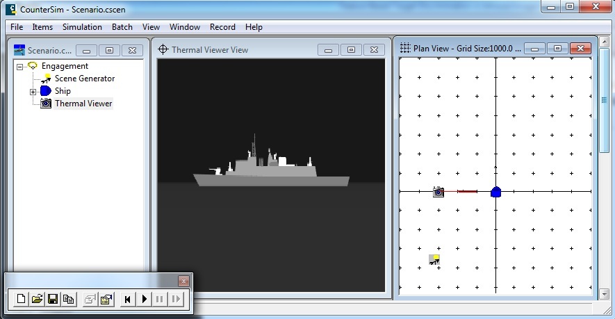
The scenario consists of an infrared imager (or thermal viewer) and a ship, which are placed at positions in (x,y,z) space as shown in the window labelled “Plan View” in Figure 1. The ship is defined by a characteristic thermal signature, applied to a three dimensional wireframe model. The imager detector resolution, field of view and waveband of operation may be specified. The imager’s view, shown in the window labelled “Thermal Viewer View” in Figure 1, may be recorded to an Audio Video Interleave file. The resulting series of images may then be processed in greyscale format using algorithms written in Matlab.

We consider four different ships for possible automatic identification: three different frigates and a corvette. To clarify, we are not attempting to classify the ships in the sense of frigate versus corvette. We are attempting to identify a ship as one of four possible ships: Frigate A, Frigate B, Frigate C or Corvette A. The ships are modelled on existing classes of frigates and corvettes, but we have given them the generic names listed.

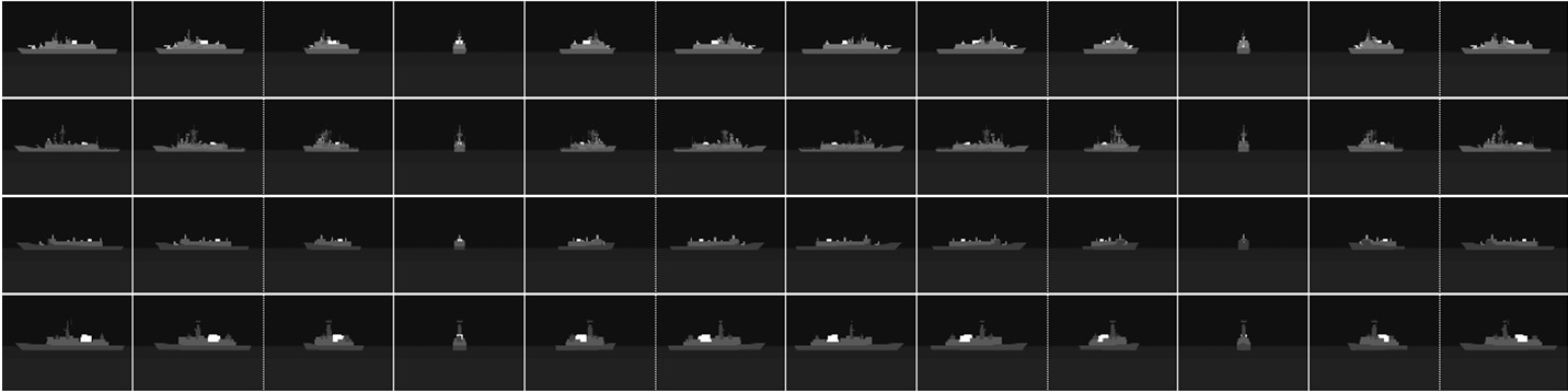
The ships are of different sizes, and so, to ensure that they each fill approximately the same field of regard in the images in the model database, they are placed at different ranges from the thermal viewer in CounterSim: Frigate A at 2700m, Frigate B at 3000m, Frigate C at 3000m, and Corvette A at 1800m. These distances are chosen so that the ships fill approximately the same area when side-on to the viewer. A model database of images of the ships at these ranges is then created, which we use to identify ships in consequent test images. The model database consists of images of the four ships generated with a varying imager-ship line of sight, in steps of 30° in azimuth, and can be seen in Figure 2. Each image in the model database is labelled with its ship name.

A database of test images is similarly created with the ships at the ranges specified for the model database, however images are now generated as the imager is moved in 10° azimuthal steps around each target. Three additional imager-ship distances of 3000m, 5000m and 7000m are considered, and 10° azimuthal sweeps are performed for all ships at each of these distances. This yields four test databases in total: one where all four ships are at the same range from the thermal imager as in the model database, and three where all four ships are at 3000m, 5000m and 7000m respectively, from the thermal viewer. Because these test databases each contain 36 images per ship, and thus 144 images in total, they are not shown here.

The scale-invariant feature transform

As discussed in the related work section, local feature detectors have become popular within the computer vision community for use in applications related to object recognition. The detectors extract local object features in images that are used to define object models. These models may be used to locate the same object in different poses in subsequent test images. Such local features have advantages over the traditional global features used for recognition in the past, in that they are more robust to partial occlusions [21].

The features, which are also referred to as keypoints or interest points, exhibit some salient property, such as being high contrast regions of the image, for instance, described by changes in image intensity. A descriptor vector may also be calculated, which characterizes the image information in a small neighbourhood around each interest point [21].

It is important for unconstrained object recognition that the interest points used to define object models remain stable under illumination and scale changes, as well as under the addition of image noise, in order to be a viable tool for use under real-world conditions.

A derivation of interest points which has become very popular in the literature, due to its robustness under the above mentioned perturbations is the Scale Invariant Feature Transform (SIFT) [23], which uses the concept of scale space theory to obtain keypoints at different scales in an image. A full derivation of the method used to obtain SIFT features and descriptors is beyond the scope of this paper, and may be found in [23], however a brief description is included here.

Keypoint locations are defined as extrema of a Difference-of-Gaussian function applied at varying scales to the image under consideration. Low contrast candidate points, and those along edges are rejected. An orientation is assigned to each keypoint, based on dominant directions of local image gradients. An orientation invariant region descriptor is compiled from the intensity gradient orientations in a region around each keypoint, which is partitioned into 16 4 by 4 pixel sub-regions. Each sub-region’s orientations are accumulated into an 8-bin histogram, and the concatenation of all 16 histograms forms the descriptor, a one-dimensional vector of length 128.

Detection of sift features and descriptors

In order to define object models for each of our four ships (Frigate A, B, C and Corvette A), we obtain SIFT features and descriptors [27] for each of the model database images introduced in the section dedicated to model and test database generation. Thus, for every model (and test) image, we obtain a set of features each consisting of a position within the image (x, y), a scale s and an orientation θ, with a corresponding set of descriptors each of dimension 128. We use these descriptors to identify the type of ship present in a test image using a Euclidean distance-based descriptor matching algorithm, and the Generalised Hough Transform for pose clustering in a similar manner to [23]. These techniques are briefly described in the following two sections, but a detailed explanation of both can be found in [23].

Descriptor matching

Suppose we have a set of descriptors obtained from a test image, and a set of descriptors from a model image. We may then find matches between the two sets using a Euclidean distance measure. The best candidate match for a test descriptor in the test image is found by identifying its nearest neighbour in the set of descriptors from the model image. The nearest neighbour is defined as the model descriptor with a minimum Euclidean distance from the given test descriptor.

A match is deemed correct if the test descriptor distance to its closest neighbour, multiplied by a value, is less than the distance to all other descriptors. If this is not the case, no match is made between the candidate test descriptor and the set of descriptors in the current model image.

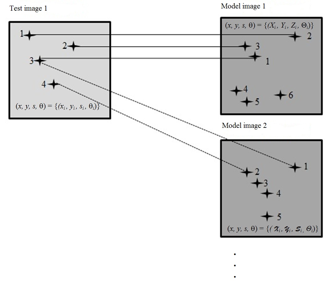
This matching process is repeated for all the descriptors in the test image under consideration, resulting in a test feature set with its corresponding matching model features. The same matching procedure is followed between a single test image and all of the model images, giving for every test image, a list of matching features for every model image, see Figure 3 for a graphical representation.

According to [23], at least three feature matches are required for reliable identification, so, two feature checks are performed for each test image. Firstly, if the number of available features that the current test image contains is less than three, then no matching to the model database is attempted, and the test image is labelled “Identification not attempted”. Secondly, for a test image, if the number of feature matches to any model image is less than three, then that model image is ignored in the list of matching features.

The generalised hough transform for pose clustering

The best match between the test image and all model images could be defined as the model image with the most feature matches to the test image. However, the presence of spurious matches (or feature match outliers) between test image features and model image features which are not related, could influence the identification process detrimentally. Thus, to reduce the effect of outlying feature matches, pose clustering via the Generalised Hough Transform [23,25,28–30] can be used. Correct matches may be separated from all matches (including false ones), by finding groups of feature matches that vote for a similar object pose. The matches that do not belong to such groups are then rejected.

For each of the matching features between a test image and a model image obtained in the previous section, there will be a similarity transformation, which links each test feature to its matching model feature. A coarse-binned histogram may then be defined in transformation parameter space. Each test-model feature match votes for its transformation within the histogram. The bin entry in the histogram with the maximum votes defines the most likely transformation between test features and model features. The feature matches in the histogram bin with the most votes are points that share a consistent transformation between the test image and the model image, and thus should belong to a single object. These feature matches will be referred to as consistent feature matches in the remainder of the document.

To identify our candidate test image, we create a separate Hough histogram for the feature matches between the test image and each of the model images, and find the most likely transformation defined by the histogram bin with the most votes. This process results in a number of votes, or vote weight for each of the model images. Finally, the model image with the overall maximum vote weight is then declared the winner. The test image is identified as the object in the winning model image.

Results

Table 1 shows how well Frigate A is identified in each of the four test databases of different range described in the section on model and test database generation. Each row of the table corresponds to a different range test database. The columns indicate the number of times that Frigate A is identified as “Frigate A”, “Frigate B”, “Frigate C”, “Corvette A”, “No identification” and “Identification not attempted” respectively. Tables 2–4 show how well Frigate B, Frigate C and Corvette A respectively, are identified in each of the four range test databases.

To understand the cause of the incorrect identifications in the tables, we must first note that a test image of a ship of type j may be incorrectly identified in three distinct ways. Firstly, misidentification type 1 occurs if there are less than three features generated in the test image, so that identification is not attempted. Secondly, misidentification type 2 occurs if a model image of a ship that is not of type j has the most consistent feature matches to the test image. If this occurs then the test image will be identified as the wrong ship type. Thirdly, misidentification type 3 occurs if less than three matches are made between the test image and any of the model images, so that the test image is identified as having “No identification”.

Test database 1: model database range

It can be seen that for the test database at the same range as the model database (row one in Tables 1–4) excellent identification accuracy is achieved: Frigate A, B and C have 35 out of 36 correct identifications, and Corvette A has 36 out of 36.

Considering row one of Table 1, it can be seen that Frigate A has one misidentification of type 2. The test image of Frigate A, generated with a viewer-ship line of sight angle of 260°, is incorrectly identified as Frigate C. This is because a model image of Frigate C has more consistent feature matches to this image than any of the model images of Frigate A. Similarly, considering row one of Table 2, Frigate B also has one misidentification of type 2 to Frigate C. These type 2 misidentifications are explained in the next paragraph.

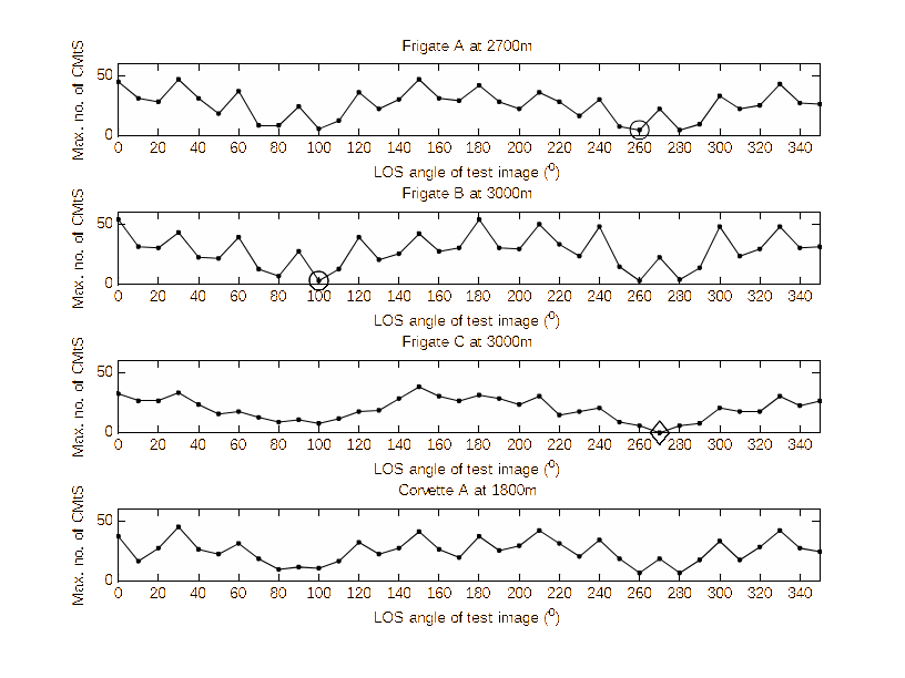
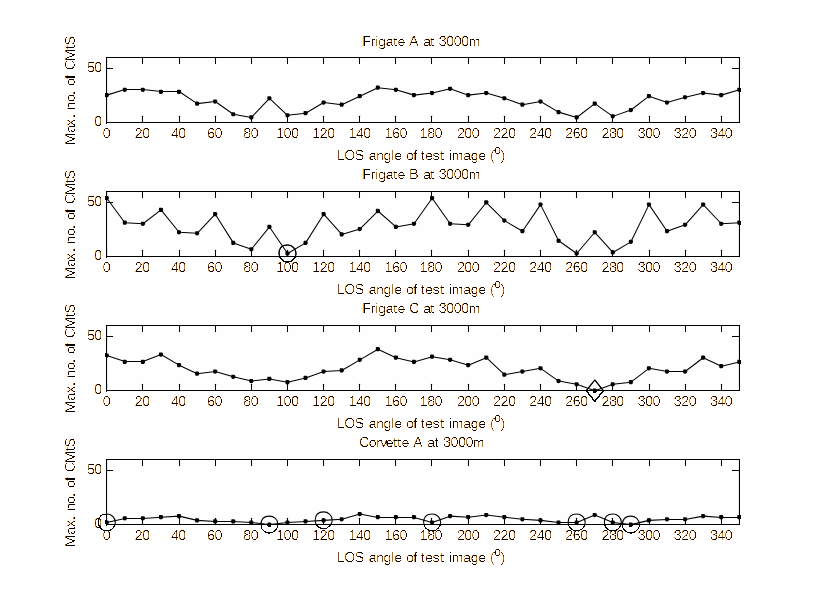
For a single test image in test database 1 we may calculate the number of consistent feature matches to all the model images that are of the correct ship type, yielding an array of number of consistent feature matches to self (CMtS). The maximum in this array is the number of consistent feature matches to the most likely model image of the ship in its own class. A plot of maximum number of CMtS for every test image is shown in Figure 4, for each of the four ship types. It can be seen that the type 2 misidentifications (marked with a circle) occur when the maximum number of CMtS are at their lowest values. These low values of maximum number of CMtS do not always imply misidentifications, since similar maximum CMtS values are obtained at other test image line of sight angles that are correctly identified. The maximum number of CMtS needs to be lower than the maximum number of consistent matches to others (CMtO) for a misidentification of type 2 to occur, and this is more likely when the maximum number of CMtS is low.

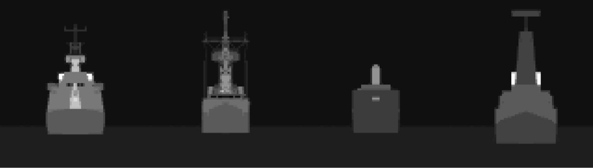
Considering row 1 of Table 3, it can be seen that Frigate C has one misidentification of type 1, where identification not is attempted. This is because only two features are generated in the image of Frigate C with a viewer-ship line of sight angle of 270°. The wireframe model used in CounterSim to generate the images of Frigate C has much less detail than the other three ships so that, on average, less features are generated in the images of Frigate C than all the other ships. In particular, the image of Frigate C with a viewer-ship line of sight angle of 270° has very little detail at all resulting in the generation of too few features for identification to be attempted. Figure 5 shows the four ships with a viewer-ship line of sight angle of 270°, showing Frigate C’s lack of detail in comparison to the other ships.

Test database 2: viewer-ship range 3000m

Considering the test database with the ships at a range of 3000m, (row two in Tables 1–4) it can be seen that Frigate A has 36 out of 36 correct identifications. For Frigate B and C, 3000m is the same range as the model database’s range so their identification statistics are the same as row 1 (35 out of 36).

In relation to the frigates, Corvette A’s correct identification rate is much worse at 3000m, at 29 correct out of 36. This is because Corvette A is much smaller than the frigates, as can be seen in Figure 6. Corvette A covers approximately the same area in images at 3000m as the frigates do when viewed from 5000m. In general, misidentification increases as ship-imager range increases, since the ships become smaller and object detail is reduced, as are available features. All of Corvette A’s misidentifications are of type 2, and occur when the maximum number of consistent matches to self is low, as can be seen in Figure 7. Notice how much lower Corvette A’s number of maximum CMtS values are in comparison to the other ships, because of its smaller size.

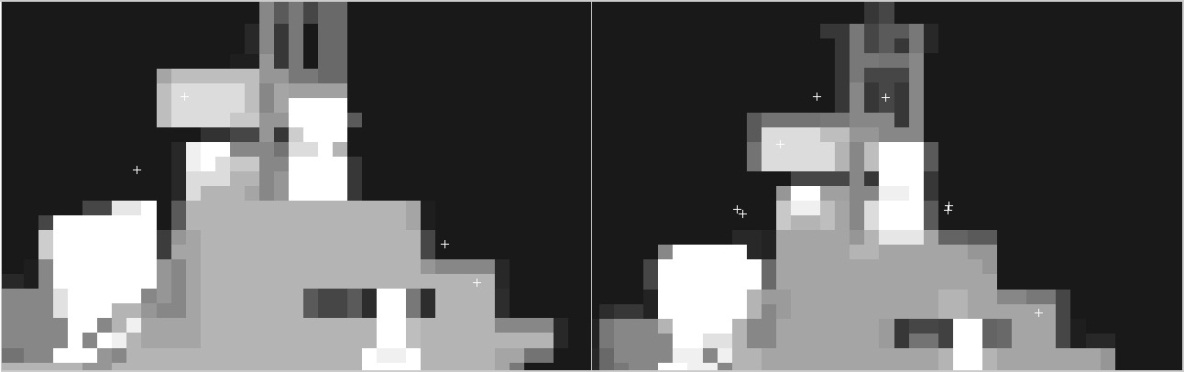
Although misidentification increases as range increases in general, Frigate A has one misidentification at 2700m and none at 3000m. This is because the distance increase is not large, and the random nature of the rendering process in CounterSim results in more texture in some areas of the image of Frigate A at a range of 3000m. This results in the generation of alternative features that consistently match better to self than to others. An example of Frigate A’s increased texture at 3000m can be seen in Figure 8.

Test database 3: viewer-ship range 5000m

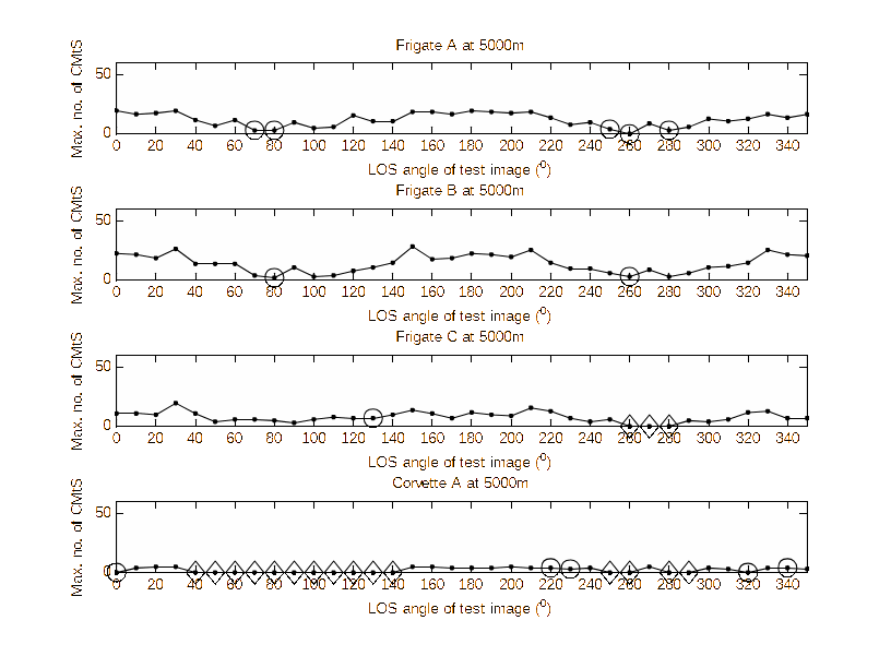
Considering the test database with the ships at a range of 5000m, (row three in Tables 1–4) it can be seen that Frigate A has 31 out of 36 correct identifications, Frigate B has 34, Frigate C has 32 and Corvette A has 16. Again, Corvette A fairs worse than the others because of its size. Fifteen out of the twenty incorrect identifications for Corvette A are of type 1: identification not attempted, where fewer than three features are generated in the test images. The remaining five misidentifications are of type 2, occurring when the maximum number of consistent matches to self is low, as can be seen in Figure 9. The maximum number of CMtS is four or less in all of Corvette A’s test images.

Frigate C has three type 1 misidentifications where no identification is attempted. These occur because of lack of ship detail in the same way as explained in the section dedicated to test database 1.

Finally, Frigate A and B have only type 2 misidentifications, occurring when the maximum number of consistent feature matches to self is low, as can be seen in Figure 9.

At 7000m, we are too far away from Corvette A to identify it. Out of the 36 test images of the corvette, 24 have less than 3 generated features, so that identification is not attempted 67% of the time. In the remaining twelve images where identification is attempted, only three features are generated per test image, Two of these images have less than three feature matches to any of the model images, resulting in an identification of type 3, or “No identification”. Only two identifications are correct.

Because of the lack of detail in Frigate C’s wireframe model, it has test images where identification is not attempted, as before. Because of the increase in viewing distance, there is a noticeable increase in these type 1 misidentifications. The average number of generated features in Frigate C’s test images, four, is low in comparison to the average values of 9 and 11 for Frigate A and B.

Frigate B’s correct identification rate is still relatively good at this range, at 30 correct identifications out of 36, or 83%. This is because Frigate B has the highest fidelity wireframe model out of all of the ships. Evidence of this can be seen in Figure 5.

Averaging over all ranges, the following percentage identification accuracy is achieved: Frigate A – 89%, Frigate B – 93%, Frigate C – 88%, Corvette A – 58%. This suggests that large ships may be identified relatively well (with greater than 80% accuracy) over large distances, given a noise free sensor, no illumination changes, and assuming the image generation process is close enough to reality. The poor results for the corvette suggest that identification should not be attempted unless the size of the target in test images is above a threshold.

Test database 4: viewer-ship range 7000m

Inclusion of thermal noise

As a simplified first attempt to investigate the effect of sensor noise on the identification process, we will consider the inclusion of thermal noise in the test images. Thermal noise in infrared sensors can be effectively modelled as Gaussian [31]. Thus, white Gaussian noise with zero mean and a variance of approximately 3% of the mean image intensity may be added to the images in the test databases described earlier. An example image can be seen in Figure 11.

Table 5 shows how well Frigate A is identified in each of the four range test databases when Gaussian noise is added to the test images. Each row of the table corresponds to a different test database range. The columns indicate the number of times that Frigate A is identified as “Frigate A”, “Frigate B”, “Frigate C”, “Corvette A”, “No identification” and “Identification not attempted” respectively.

Tables 6–8 show how well Frigate B, Frigate C and Corvette A respectively, are identified in each of the four range test databases with Gaussian noise added. The addition of noise causes the generation of spurious additional features in the test images, and consequently no type 1 misidentifications occur, where less than three features are generated in a test image and identification is not attempted.

Averaging over all ranges the following percentage identification accuracy is achieved: Frigate A – 81%, Frigate B – 81%, Frigate C – 79%, Corvette A – 49% with an increase overall of 12 misidentifications for Frigate A, Frigate C and Corvette A, and an increase of 17 for Frigate B. The increase in misidentifications is because of a reduction in the maximum number of consistent matches to self in the majority of all of the test images, as a result of the noise.

Ignoring the test database with images generated at viewer-ship range 7000m, the overall identification results for the large ships are Frigate A – 89%, Frigate B – 86% and Frigate C – 89%, which are of the same order of magnitude as the overall results with no noise. This suggests that the inclusion of noise reduces the identification range of the large ships by around 2000m.

Illumination changes

Illumination changes to the scenes rendered in CounterSim may be introduced by the usage of sun-like spotlights, an example image of which can be seen in Figure 11. Four new test databases may be created including such illumination, with the ships at (1) the ranges specified for the model database, (2) at viewer-ship ranges of 3000m, (3) at viewer-ship ranges of 5000m and (4) at viewer-ship ranges of 7000m.

Table 9 shows how well Frigate A is identified in each of the four range test databases when sun-like spotlights change illumination in the test images. Each row of the table corresponds to a different test database range. The columns indicate the number of times that Frigate A is identified as “Frigate A”, “Frigate B”, “Frigate C”, “Corvette A”, “No identification” and “Identification not attempted” respectively. Tables 10–12 show how well Frigate B, Frigate C and Corvette A respectively, are identified in each of the four range test databases with changes in illumination in the test images.

Averaging over all ranges, the following percentage identification accuracy is achieved: Frigate A – 81%, Frigate B – 89%, Frigate C – 76% and Corvette A – 45%. There is an increase overall of 11 misidentifications for Frigate A, 6 for Frigate B, 17 for Frigate C and 18 for Corvette A.

Frigate B’s identification accuracy is the least affected by the sun-like spotlight, since the facets of its wireframe model are small, and as a consequence, areas of high, constant solar reflection are smaller than the other less complicated ship models with larger facets. Evidence of this can be seen in Figure 12.

SIFT descriptors are designed [23] to be invariant to the effects of affine (additive or multiplicative) changes in illumination that are the same over the entire image, as they are normalised to unit length. The effect of non-linear illumination changes are reduced [23] by thresholding the values in the descriptor vector to 0.2, and then renormalizing. The value of 0.2 is determined experimentally in [23], and is used in our experiments; however, because of the bias towards low intensity pixels in our test images, this threshold value may need to be re-determined.

Ignoring the test database with images generated at viewer-ship range 7000m, in the same way as before gives the overall identification results for the large ships as: Frigate A – 90%, Frigate B – 95%, Frigate C – 87%, implying that illumination changes yield a similar reduction in the identification range of the large ships.

Simulation parameters

All results in this paper were generated [27] using the SIFT scale parameters of six octaves and three intervals as in [23].

In the section dedicated to the Scale Invariant Feature Transform, it was explained that low contrast candidate keypoints are rejected. This is achieved by setting a contrast threshold parameter in [27], so that candidate points with a contrast less than the threshold are excluded. This prevents the inclusion of non-ship features triggered by the background sky and sea in the model and test database images. A threshold value of 0.0065 was used in the generation of all results. The multiplicative value used in descriptor matching when comparing the nearest neighbour to all other matches was 1.5.

Conclusion

This paper considers the task of object recognition for the possible introduction of target discrimination capabilities in unmanned aircraft. We are concerned with a naval scenario, and attempt to identify automatically four different ships in simulated infrared imagery, using a feature detector: SIFT, which is popular within the computer vision community.

Our results show that the features generated by the Scale Invariant Feature Transform are robust to variations in scene illumination and the inclusion of Gaussian noise in the simulated infrared images. We also see that sensor range from the target can be a debilitating factor in identification accuracy.

The current work is limited by the size of the model database, which only contains four different ship classes at a single range with varying azimuth view angle. Images generated with varying pitch angle should be included in the model database in further work, as well as investigating the inclusion of a number of different ranges for each of the different ship types. This may improve identification at different ranges. Ideally, the database should include many more ship classes (more than 1000 if only considering military vessels, according to [32]). The author is aware that this will have a detrimental effect on the speed of target identification.

Current identification times (not including the time taken for interest point generation and matching) are already of the order of 0.2 seconds for a test image on an Intel i5 3.2GHz processor overclocked to 4.0GHz. It should be mentioned that no code optimisation has been attempted on the Generalised Hough Transform Matlab functionality, and replacing the non-optimised code with an efficient hash table implementation as in [23] should reduce the identification time considerably. Although the SIFT interest point detector is known to be computer intensive, a Graphic Processing Unit (GPU) based real-time object recognition system using SIFT features has been reported in [33] with a database of three objects.

A second limitation on the work in this paper is the simulated infrared imagery used. Further work should attempt to validate the proposed method with actual infrared images. It should also be noted that infrared images bring their own unique challenges to the task of automatic target recognition in that high variation in the thermal signatures of targets is observed [34]. Target signatures vary considerably according to the time of day and recent history of the target [35]. Infrared images also often contain high concentrations of background clutter whose characteristics also change with environment, making target detection difficult [36]. Infrared sensors are affected by rain, fog and haze; they have poor cloud penetration and have only moderate atmospheric range [13]. Thus, it would be desirable to consider the use of a multi-sensor suite with a combination of processing algorithms when addressing the task of automatic target recognition in unmanned aircraft.

References

Authors

Greer J. Gray is a PhD student in the Department of Informatics and Systems Engineering at Cranfield University at the UK Defence Academy. Her supervisors are Dr Mark A. Richardson, and Dr Nabil Aouf. She would like to extend thanks to her supervisors, and to Brian Butters, Roy Walmsley and Edgar Nicholls at Chemring Countermeasures Ltd., her sponsor. Email may be addressed to g.gray@cranfield.ac.uk.

Dr Mark Richardson is a Reader in Electro-Optics & Infrared and is Head of the Sensors Group at the Defence Academy of the UK. Email may be addressed to m.a.richardson@cranfield.ac.uk.

Dr Nabil Aouf is a Lecturer in Signals, Imaging and Systems at Cranfield Defence and Security, at the Defence Academy of the UK. Email may be addressed to n.aouf@cranfield.ac.uk.

Brian Butters is the Manager of Modelling and Simulation at Chemring Countermeasures Ltd., and is responsible for software development and the conduct of studies of expendable countermeasure effectiveness. He is a member of the Institute of Physics and is a Chartered Physicist who has worked in the electronic warfare industry for more than thirty years. Email may be addressed to brian.butters@chemringcm.com.

Roy Walmsley gained a BSc in Chemistry from Leeds University and has over 25 years’ experience in the pyrotechnic industry, including new product development, performance testing and instrumentation and latterly simulation and modelling. Email may be addressed to roy.walmsley@chemringcm.com.

Edgar Nicholls gained a BSc in Physics from Imperial College. He currently works as a modelling and simulation engineer at Chemring Countermeasures Ltd. Email may be addressed to edgar.nicholls@chemringcm.com.

References

[1] WinterGreen Research Inc., Unmanned Aircraft Market Shares, Strategies, and Forecast, Worldwide, 2011 to 2017, 2011.
[2] B. Alkire, J.G. Kallimani, P.A. Wilson and L.R. Moore, Applications for Navy Unmanned Aircraft Systems, RAND Corporation, 2010.
[3] Naval Studies Board, Autonomous Vehicles in Support of Naval Operations, National Academies Press, 2005.
[4] G. Yeo, “Boeing Bites into Asian Pie”, Flight International, Vol. 177, No. 5245, 2010, pp. 24.
[5] L. Dickerson, “UAVs Buoyed by Defense”, Aviation Week and Space Technology, Vol. 162, No. 3, 2005, pp. 101-104.
[6] R. Austin, Unmanned Aircraft Systems: UAVS Design, Development and Deployment, John Wiley & Sons, Ltd, 2010, pp. 283, 299
[7] United States Army UAS Center of Excellence, United States Army Unmanned Aircraft Systems Roadmap 2010 to 2035, 2010.
[8] Headquarters, United States Air Force, United States Air Force Unmanned Aircraft Systems Flight Plan 2009 to 2047, 2009.
[9] BAE Systems, “First Composite Component for Taranis in Manufacture”, BAE Systems Press Release, Ref. 379/2007, 2007.
[10] United States Army, Army Unmanned Aircraft System Operations, Field Manual Interim, FMI 3-04.155, 2006.
[11] W.E. Snyder and H. Qi, Machine Vision, Cambridge University Press, 2004, pp. 392
[12] B. Bhanu, “Automatic Target Recognition: State of the Art Survey”, IEEE Transactions on Aerospace and Electronic Systems, Vol. AES-22, No. 4, 1986, pp. 364–379.
[13] B. Bhanu and T.L. Jones, “Image Understanding Research for Automatic Target Recognition”, IEEE Aerospace and Electronic Systems Magazine, Vol. 8, No. 10, 1993, pp. 15–23.
[14] D.E. Dudgeon and R.T. Lacoss, “An Overview of Automatic Target Recognition”, Lincoln Laboratory Journal, Vol. 6, No. 1, 1993.
[15] P.J. Withagen, K. Schutte, A.M. Vossepoel and M.G.J. Breuers, “Automatic Classification of Ships from Infrared (FLIR) Images”, Proceedings of SPIE, Vol. 3720, Conference on Signal Processing, Sensor Fusion, and Target Recognition VIII, 1999, pp. 180–187.
[16] C. Tremblay and P. Valin, “Experiments on Individual Classifiers and on Fusion of a Set of Classifiers”, Proceedings of the Fifth International Conference on Information Fusion, Vol. 1, 2002, pp. 272–277.
[17] J. Alves, J. Herman and N.C. Rowe, “Robust Recognition of Ship Types from an Infrared Silhouette”, Command and Control Research and Technology Symposium, 2004.
[18] Lu Jun-Wei, Ren Jian-Cun, Wang Ting, Wang Chen-Gang and Yuan Xiao-Hu, “Infrared Ship Multi-Targets Recognizing”, IMACS Multiconference on Computational Engineering in Systems Applications, 2006, pp. 418-423.
[19] Heng Li and Xinyu Wang, “Automatic Recognition of Ship Types from Infrared Images Using Support Vector Machines”, International Conference on Computer Science and Software Engineering, 2008, pp. 483–486.
[20] S.P. van den Broek, H. Bouma and M.A.C. Degache, “Discriminating Small Extended Targets at Sea from Clutter and Other Classes of Boats in Infrared and Visual Light Imagery”, Proceedings of SPIE, Signal and Data Processing of Small Targets, Vol. 6969, 2008.
[21] M. Treiber, An Introduction to Object Recognition, Selected Algorithms for a Wide Variety of Applications, Springer-Verlag London Ltd, 2010.
[22] T. Tuytelaars and K. Mikolajczyk, “Local Invariant Feature Detectors: a Survey”, Foundations and Trends in Computer Graphics and Vision, Vol. 3, No. 3, 2008, pp. 177–280.
[23] D.G. Lowe, “Distinctive Image Features from Scale-Invariant Keypoints” International Journal of Computer Vision, Vol. 60, No. 2, 2004, pp. 91-110.
[24] P.A. Feineigle, D.D. Morris and F.D. Snyder, “Ship Recognition using Optical Imagery for Harbor Surveillance”, Proceedings of Association for Unmanned Vehicle Systems International, 2007.
[25] W.E.L. Grimson and D. Huttenlocher, “On the Sensitivity of the Hough Transform for Object Recognition”, AI Memos, Vol. 1044, 1988.
[26] Chemring Countermeasures Ltd., Modelling and Simulation, http://www.chemringcm.com, last accessed 13 June 2011.
[27] A. Vedaldi and B. Fulkerson, VLFeat: An Open and Portable Library of Computer Vision Algorithms (ver. 0.9.9), 2008, http://www.vlfeat.org, last accessed 13 June 2011.
[28] P.V.C. Hough, Method and Means for Recognizing Complex Patterns, U. S. Patent, 3069654, 1962.
[29] D.H. Ballard, “Generalizing the Hough Transform to Detect Arbitrary Shapes” Pattern Recognition, Vol. 13, No. 2, 1981, pp. 111-122.
[30] T.F. El-Maraghi, Hough Transform Functionality in Matlab Sift Tutorial, 2004, Department of Computer Science, University of Toronto, ftp://ftp.cs.utoronto.ca/pub/jepson/ teaching/vision/2503/SIFTtutorial.zip, last accessed 13 June 2011.
[31] J.M. Palmer and B.G. Grant, The Art of Radiometry, SPIE Press, 2009, pp. 135.
[32] A.E. de Luna, C. Miravet, D. Otaduy and C. Dorronsoro, “A Decision Support System for Ship Identification Based on the Curvature Scale Space Representation”, SPIE Proceedings Vol. 5988, Electro-Optical Remote Sensing, 2005
[33] G. Hsu, C. Lin and J. Wu, “Real-Time 3-D Object Recognition Using Scale Invariant Feature Transform and Stereo Vision”, 4th International Conference on Autonomous Robots and Agents, 2009, pp. 239–244.
[34] V.M. Patel, N.M. Nasrabadi and R. Chellappa, “Automatic Target Recognition Based on Simultaneous Sparse Representation”, 17th IEEE International Conference on Image Processing, 2010, pp. 1377—1380.
[35] W.M. Brown and C.W. Swonger, “A Prospectus for Automatic Target Recognition”, IEEE Transactions on Aerospace and Electronic Systems, Vol. 25, No. 3, 1989, pp. 401—410.
[36] V.M. Patel, N.M. Nasrabadi and R. Chellappa, “Sparsity-Motivated Automatic Target Recognition”, Applied Optics, Vol. 50, Apr, 2011, pp. 1425–1433