Mie Lidar: Instrument Description And Applications

Introduction

There have been a number of uses of toxic chemicals (chemical and biological warfare agents) against civilian and military targets by terrorists and rogue countries [1–4]. Toxic chemicals in vapour form start dispersing as soon as they are released in the atmosphere and form small-stratified layers/clouds in the lower troposphere due to background atmospheric wind speed. The lifetime of these clouds can be from an hour to a day, depending upon their nature. In the course of time these toxic clouds settle down, thereby causing a health hazard to plants, animals, and human beings. These incidents have increased worldwide awareness of early detection of chemical agents in the atmosphere. Specifically, the standoff detection and detection time are very important for threatened personnel to take defensive or preventive measures against such a threat. Detecting such tenuous thin layers of toxic chemicals, and their spatial and temporal distribution along with the measurement on their optical properties is a challenging task. LIDAR (light detection and ranging) is the only realistic method for standoff detection of toxic agent today and uses lasers as excitation source [5–7].

LIDAR transmits a high-peak-power laser pulse into the atmosphere, which interacts with the atmospheric constituents causing alterations in the intensity, polarization and wavelength of the backscattered light. From the measurement of these parameters of the received light, one can deduce the properties of the aerosols and other minor constituents of the atmosphere [8–10]. The distance to the scattering medium can be deduced with very high accuracy from the time delay of the return signal. LIDAR systems are used in the wavelength range starting from ultraviolet (UV) to the mid infrared (mid-IR) by using different types of lasers [11−13]. LIDAR systems are superior to point detection systems (such as infrared spectrometry, Raman spectrometry, and FTIR) because of their capability of ranging and discriminating between the various molecules in real time. The detection method can be based on several physical phenomena. The most common phenomena are elastic backscattering, laser induced fluorescence and differential absorption. The backscattering LIDAR with proper combination of pulse energy, pulse repetition frequency and suitable receiver optics can differentiate the chemical or biological cloud return signals from the background atmosphere. It is expected that this system could detect the presence of chemical and biological clouds at distances of a few kilometres depending on the cloud concentration and weather conditions. Further, it can discriminate between the composition of toxic clouds based on the concept of differential absorption and fluorescence [12,13].

The Laser Science and Technology Centre (LASTEC), Delhi, has been working on a project to develop a multi-wavelength LIDAR system for detection of chemical and biological warfare agents. As a part of main LIDAR activities, a backscattering LIDAR system based on the Mie scattering principle has been designed operating at 1064 nm. This has the capability of detecting remotely the cloud structures formed by aerosols, water vapour or toxic materials in the atmosphere though it cannot identify its composition and concentration. The measurement of depolarization of the signal is also incorporated to study the nature of the scattering particulates. In this paper, we report the technical details of the LIDAR system and discuss some of the preliminary experimental results. Results presented in this paper pertain to the data taken during the day time.

System details

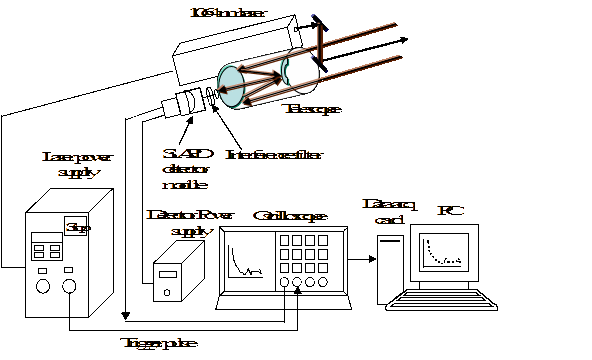
The LIDAR system uses a pulsed Nd:YAG laser (Surelite I-10 Laser from Continuum, USA) emitting at the fundamental wavelength of 1064 nm, as the main transmitting source. Laser pulse energy is variable from 25 mJ to 400 mJ. The pulse width of the laser is 7 ns and its pulse repetition frequency is 10 Hz. The laser beam diameter is 6 mm at the output aperture and has a divergence of 0.6 mrad. The system is configured in a coaxial mode by folding the laser beam using two reflective mirrors so that the laser beam enters the field of view of a telescope. Figure 1 describes the block diagram of experimental setup. This setup is installed on a movable tripod stand, which is manually controlled. This tripod stand is designed and fabricated in-house. It can scan the atmosphere in 360° in azimuth and –10° to 45° in elevation. The scattered radiation from the atmosphere is collected by the 200 mm diameter Cassegrain telescope and its field of view is less than 3 mrad. A passband interference filter with bandwidth (FWHM) of 3 nm centred on the laser wavelength is used to reduce the atmospheric background noise. The IR optical signal from the telescope is focused onto a high quantum efficiency Si: avalanche photo diode (APD) detector module (Licel, Germany). The Si:APD module consists of an integrated TE cooler and temperature controller, preamplifier, focusing lens and HV power supply. NI’s PCI bus based DAQ card is used as data acquisition hardware in this system.

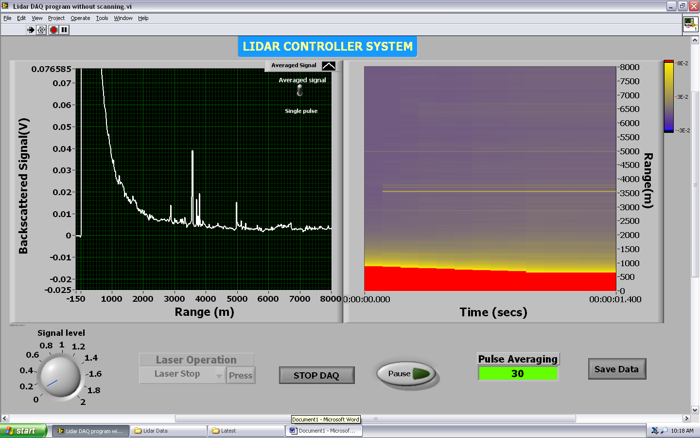
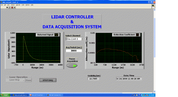
The return signal from the detector is connected to an analogue input channel of the DAQ and the trigger signal from the laser source is connected to the digital trigger input of the card. The DAQ is configured to a sampling rate of 10 MHz to have a range resolution of 15m, which corresponds to 0.1 µsec. The number of samples is set to 500 so as to collect data up to a range of 7.5 km. Figure 2 shows the LIDAR controller software developed in-house in LabView used to control the laser source and data acquisition hardware. The laser system is switched on by invoking controls in the user interface and it starts firing pulses at a rate of 10 Hz. The data acquisition process is started when the start DAQ button is pressed in the Graphical User Interface and data for every 500 samples at 15 m range bins is stored to the computer hard disk for every laser pulse transmitted. A typical backscattered signal versus range is presented on left side of the panel in Figure 2. The backscattered signals from the atmosphere were collected from the near field to maximum range of 7–8 km. The Si:APD signal reached a maximum value of about 1,100 mV, which is the saturation level of the detector. Thereafter, the signal started falling steadily with respect to range. It showed clearly that the experimentally measured multiple cloud signals (cloud signal strength is higher than the background signal) at a distance of 3.5 km and 5 km. the image shown in the right side of the panel in Figure 2 represents the temporal variation of the received signals. Signals received from the nearby region are very strong and accordingly a colour coding is assigned (red-strong signals and blue-weak signals). From the LIDAR signal information pertaining to the various parameters such as extinction coefficient, visibility has also been obtained by using suitable LIDAR inversion methods in real time. The complete LIDAR system is connected to a UPS system, which can keep the LIDAR operational with captive power for nearly one hour. Table 1 presents the technical details of the LIDAR system. This system has been tested and validated by measuring return signals from atmospheric aerosols and clouds in real time under different atmospheric conditions. Some of the measured signals are processed for further investigation and results are discussed in the subsequent sections.

Signal processing

From the LIDAR signal, information pertaining to the various parameters has been obtained by using the suitable LIDAR inversion methods. The single scattering equation for a monostatic pulsed LIDAR may be written as:

where P(R) is the received signal at range R, P_t is the transmitted power, η summarizes all system constants such as optical efficiency, and detection efficiency. β(R) is the volume backscattering coefficient of aerosols (β_a(R)) and air molecules (β_g(R)), α(R) is the volume extinction coefficient of aerosols (α_a(R)) and air molecules (α_g(R)), c is the speed of light, and τ is the pulse duration. This equation indicates that in a homogeneous atmosphere, P(R)×R² decreases with range as an exponential function. In the presence of a cloud layer, the signal level undergoes a rapid increase because of enhanced backscattering of cloud droplets, and then reaches its maximum value before decreasing to the level of backscatter from ambient air or disappearing into the background noise level. Klett [14] developed the backward inversion method using the analytical solution of the single scattering LIDAR equation shown in (1). To invert (1), another relationship between the two unknowns α and β is needed. These two coefficients are dependent on the nature of the scattering particles. The relation between these two parameters [14] is:

where constants C and k depend on the LIDAR wavelength and various properties of the aerosol particles. Constants, k≈1 and C≈0.05 sr^-–1 [15] appear to be the values most often reported. They are generally taken to be constant over the optical path. The LIDAR equation (1) is solved with the use of (2) to obtain the final backward integration equation to derive the atmospheric extinction coefficient, which is:

The boundary value α_m is chosen at the far end near the maximum range R_m at which a usable signal is available before it reaches the constant background noise level (α_m = α(R_m)). The advantage of this method is the fact that the system constant no longer has to be determined. However, a drawback of this technique is to have a boundary value at the far end range R which is, in general, more difficult to obtain than that at the near range R. However, Klett [14] was able to show that the influence of α_m on the resulting α(r) profile decreases strongly with the optical depth between R and R_m. We have assumed a typical value in the order of 10^–5 m^–1 as a reference value to invert the LIDAR signal downward from range of 5 km. The influence of incorrect starting value is mainly limited to the far end (last third) of the measurement path. The first two-thirds of the inverted measurement path can be seen as very good estimates. The reason for this is that the second term in the denominator of (3) rapidly becomes large compared with the first term, especially for large boundary values of α_m. Hence, evaluating the LIDAR profile for a cloudy and foggy atmosphere is straight forward. We also mention clearly that the backscattering-to-extinction ratio (C) is not uniform over different regions of the troposphere [16]. Detailed analysis is required to study the influence of C as a function of relative humidity of the atmosphere and aerosol composition over Delhi. In our analysis, we assumed a uniform C over the entire range and have not incorporated multiple scattering factors in our analysis.

Applications

Determination of aerosol extinction coefficient

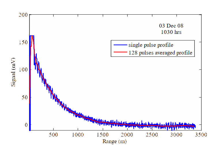
Experiments were conducted using this system under different atmospheric conditions ranging from clear sky conditions to a cloudy and overcast sky. A laser beam with pulse energy of 50 mJ was transmitted into the atmosphere at an elevation angle of 12° along the slant path. Since most of the experiments were conducted during daytime, regular monitoring of the sky condition was carried our visually. The backscattered signals from the atmosphere were collected from the near field to a maximum detectable range of up to 7–8 km using this system. Figure 3 shows a typical example of the LIDAR signal obtained in the experiment conducted on a clear day (winter month 3 December 2008, 15:30 hrs local time). Due to strong sky background noise we would see the fluctuations in the return signals across the entire range. The return signals do not show any significant variation with respect to distance beyond 2 km, in other words the signal merges with background noise levels. The fluctuations in the LIDAR signal can be overcome easily by averaging a larger number of pulses. However, for our studies a total number of 128 pulses were averaged to obtain a single noise free smooth signal profile. We have also applied spatial moving averaging of 10 to 20 samples to remove random noise depending upon the signal behaviour (Figure 3).

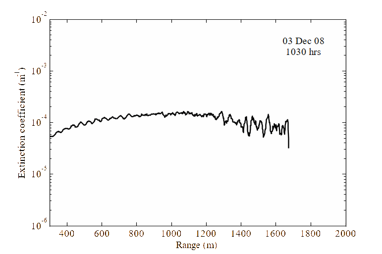
The aerosol extinction coefficient profile was derived using the method described earlier. The exponent k in (3) was set to unity since the resulting profile depends only weakly on k. Figure 3 describes the aerosol extinction coefficient obtained for single pulse along slant path. Extinction coefficient values mostly varied between 6.52×10^–5 m^–1 and 1.21×10^–4 m^–1. Results are in good agreement with the reported literature values [17]. It can be seen that extinction values do not show much variations along the slant path. This is due to the fact that the laser beam travels in the homogeneous region of the atmosphere.

Detection of atmospheric clouds

One of the potential applications of LIDAR is in the studies of characterization of clouds. Usually strong backscattering arises from clouds due to the relatively large scattering cross-sections of cloud particles and the huge number density of scatterers. The same experimental set-up was used for detection of clouds in the atmosphere. In general, we inspected the sky condition visually before firing the laser beam into the atmosphere. The first information on the presence of a cloud is obtained by simply looking at the signal profile with altitude in the visual display on the oscilloscope and the computer. The LIDAR data shows a sudden upsurge in signal strength where the clouds are present from its normal fall with range in the presence of background aerosols. The visual display gives clearly a qualitative nature of the cloud layer indicating its altitude and information whether the layers are single or multiple. The presence of cloud is determined by the following quantitative criteria: (1) a sudden upsurge, (2) a rapid decrease just after a maximum, and (3) the actual value of the extinction coefficient at the peak.

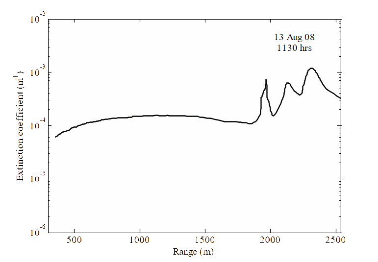
Figure 5 shows the behaviour of the LIDAR return signals obtained on 11 August 2008, 16:21 hrs from the clouds. It clearly revealed the strong return signals from the clouds in the range between 7.15 km and 7.47 km. As a case study, we have conducted an experiment on a rainy day. The backscattered signal obtained on 13 August 2008, 1130 hrs from the low level clouds is presented in the Figure 6.

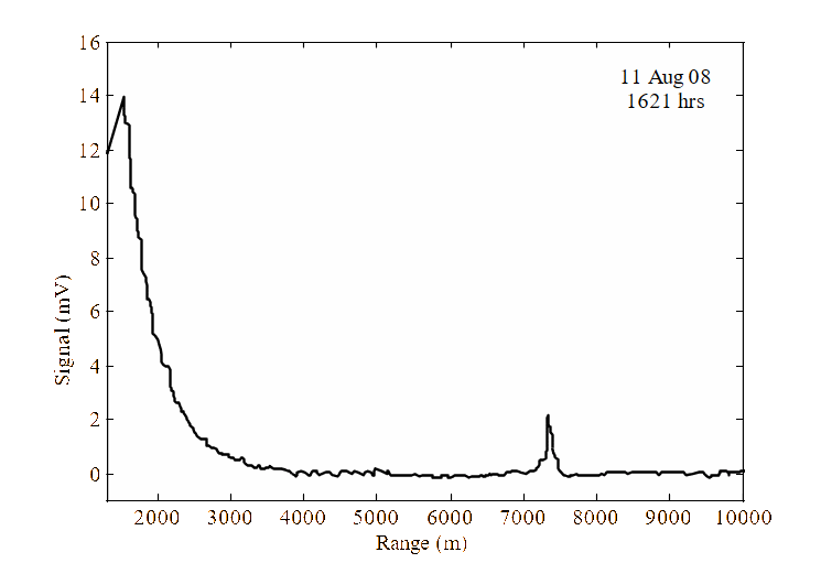
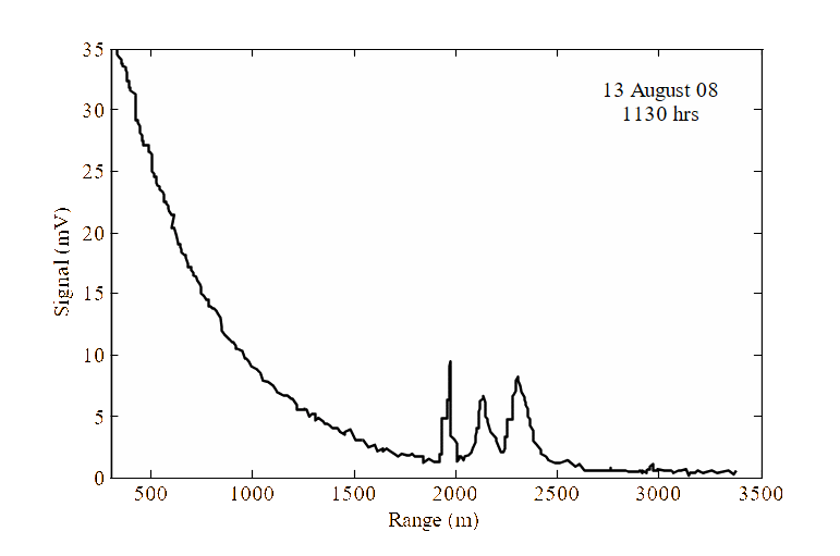
The total signal is basically characterized by the nature of cloud and other species in the atmosphere—that is, humidity, drizzle and aerosols contribute to increases in the backscattered signal. The cloud signal-to-noise ratio (SNR) is large and the retrieval of cloud heights (that is, base and top) from a single profile is not difficult. The cloud base and heights have been derived from the measured waveforms at different times. The cloud thickness is then derived from the difference between the apparent cloud top and base. The cloud was detected between the 1.87 km and 2.62 km region. The geometrical thickness of the cloud is about 550 m. Our visual inspection revealed the presence of low-level rain bearing clouds on this day and our experimental site also received intermittent rainfall.

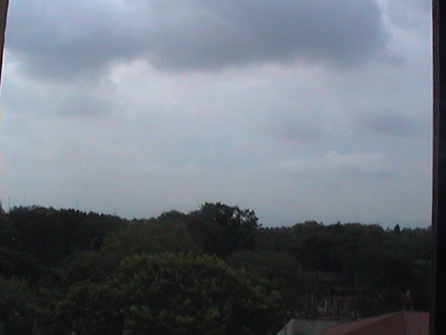
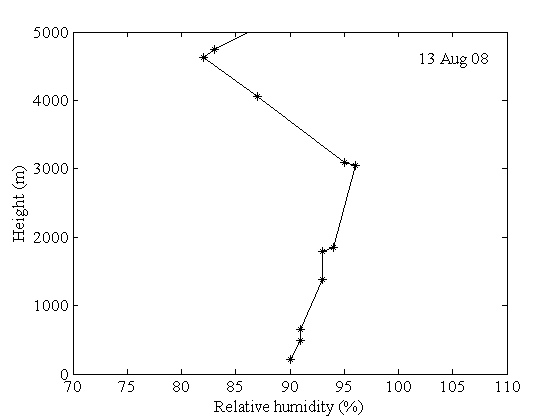
An image of the sky condition was captured using a digital camera before the start of the experiment and is shown in the Figure 7. It clearly shows the presence of thick dark clouds. Figure 8 shows the relative humidity versus altitude obtained from the radiosonde instrument at New Delhi (http://weather.uwyo.edu/upperair/sounding.html). The relative humidity of more than 90% even up to a maximum altitude of 4 km confirmed the presence of low level clouds (water vapor present in the atmosphere due to the increase in humidity). The extinction coefficient values are calculated for cloud signals and presented in Figure 9. The extinction coefficient, in general, falls with range in the lower troposphere and the values lie typically in the range 0.75–1.12 x10^–4 m^–1 in the absence of any cloud whereas this value increases up to the order of 10^–3 m^–1 in the presence of clouds. Enhancement in the extinction values in the cloud region reaching the peak value of about 1.26×10^–3 m^–1 were observed.

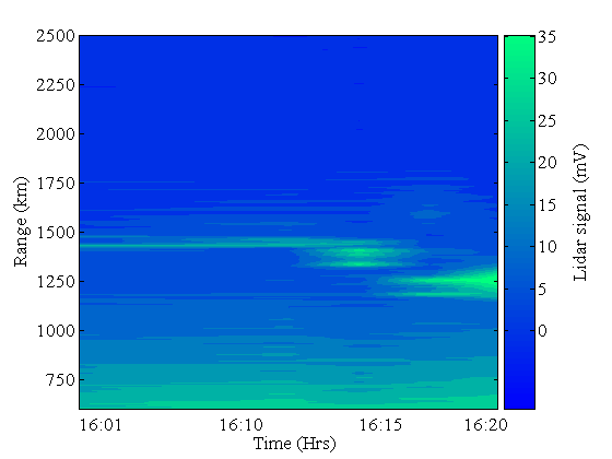
These values are in agreement with the results reported by Puchalski [18] who conducted LIDAR measurements at 1064 nm and estimated the cloud extinction coefficient for low-level thin clouds of a stratus type. Guaumet et al [19] also reported the similar phenomenon studied using a LIDAR system. Figure 10 shows the temporal variation of cloud pattern obtained on 18 Sep 2008. The system was operated for about two hours continuously. Here we presented the lidar signal obtained from 16:00 hrs to 16:20 hrs. An enhancement in signal strength is seen between 1.2 km and 1.5 km due to the presence of clouds. The cloud thickness measured at various times is changed very rapidly since the clouds were moving quickly away from the field of view of the telescope. This would be due to the prevailing thermodynamic processes within the clouds leading to changes in geometrical thickness.

Determination of visibility

LIDAR offers advantages for determining the atmospheric visibility over extended and the remote paths [20–21]. The measurement of the volume extinction coefficient (α) is the preferred approach for determining of visibility. When the atmospheric particle size distribution is unknown, empirical expressions [22–23] may be used to predict the wavelength dependence of particulate extinction. A frequently quoted empirical relation for visually clear air is:

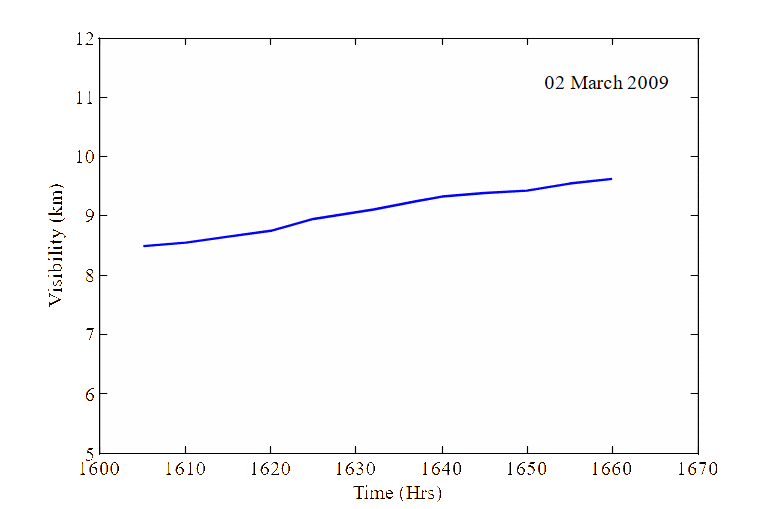
here q = 1.3 for ‘average seeing condition’, α is the mean extinction coefficient value derived from a LIDAR signal over the range interval from the near field to 2-5 km. The mean extinction coefficient value is derived from each profile over range intervals from near field to the maximum detectable range. This value is used in the above relation to calculate the atmospheric visibility at 1064 nm. The experiments were conducted for determining the visibility using the current system. The laser radiation was transmitted along the horizontal path for this purpose. The backscattered radiation was collected and processed to obtain a mean extinction coefficient using the method described earlier. Typical examples of visibility measurement are presented in Figure 11. Figure 12 illustrates the temporal variation of visibility. Data collected on 2 March 2009 during the period 16:19 hrs to 16:40 hrs was used in this calculation. It shows the increasing trend in the visibility with respect to time due to local changes in the atmospheric processes. The average visibility obtained on this day was 9.1 km.

Measurement of depolarization signal

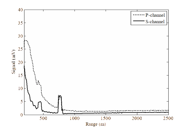
LIDAR measurements of depolarization ratio provide highly reliable information to discriminate the nature of biological aerosols in the atmosphere. The basic polarization LIDAR application involves the transmission of a linearly polarized laser pulse and detection via a beam splitter of the orthogonal and parallel planes of polarization of the backscattered light. The ratio of two signals is known as the depolarization ratio (δ). The depolarization method is used to differentiate the solid, liquid, or mixed phase of biological aerosol or clouds. Spherical particles like water droplets and air molecules cause no depolarization, so that δ~0, whereas non-spherical particles, such as ice clouds, mineral dusts, biological aerosols produce depolarization, so that δ>0. Fluorescence LIDAR coupled with depolarization measurement is suggested as one of the approaches for effective discrimination between biological aerosols and non-hazardous aerosol clouds. It has been used to measure the depolarization ratio of biosimulants (bacillus anthracis), interferent aerosol clouds released in the field using 1.54 µm [24] and 1.064 µm elastic lidar [25]. In view of the importance of depolarization measurement, an experimental set up has been established to measure the parallel and perpendicular polarized signals from the atmosphere. In the present set up, a new mechanical adaptor has been designed, fabricated and fitted at the end of the receiving telescope. This can accommodate two individual detector boxes that contain an interference filter, Si:APD detector modules and a polarizing beam splitter. The backscattered radiation from the atmosphere is allowed to pass through polarizing cube beam splitter which then separates the parallel and perpendicular polarization components before it reaches the detectors. The detected signals are passed through A/D converters and data processors for further processing. Preliminary experiments have been conducted recently to measure the depolarized signals from known near range targets. The linearly polarized laser radiation at 1064 nm with pulse energy of 50 mJ was transmitted into the atmosphere, which interacted with tree leaves. The multiple return signals from the target were measured simultaneously using two detectors. Detectors were operated at the same operating voltage in order to have the same gain at both channels. Figure 13 shows a typical example of the measured return signals at the parallel and perpendicular channels. Return signals at both detectors reduce with range after reaching the saturation level. There is an enhancement in signal strength observed at about 420m and 720m, which is due to tree leaves. The signal pattern and amplitudes are different for both detectors. This is due to the fact that the non-sphericity of the target changes the state of polarization. Further experiments are planned to measure the depolarization signals from the various targets such as biosimulants, diesel, and pollen.

Conclusion

A tripod mounted mobile Mie LIDAR system has been designed and developed at LASTEC. The transmitter energy of 50 mJ/pulse, pulse duration of 7 ns and 10 Hz, PRF has been used for the experiments. The preliminary results indicated that the LIDAR has the ability to detect clouds and lower tropospheric aerosols. The extinction coefficients for aerosols and clouds have been derived from the LIDAR-backscattered signals. LIDAR experiments also demonstrated its capability to measure the atmospheric visibility. The average visibility obtained on a particular day was 9.1 km. This system was reconfigured to measure the depolarized signals from the atmosphere. Depolarization measurement revealed the significant change in return signal in parallel and perpendicular channel detectors. The change in signal is due to the non-sphericity of the target. This LIDAR can be used for routine measurements of the distribution and variation of clouds and aerosols at sites of interest. Currently, this system is being modified for auto scanning of the atmosphere in elevation and azimuth region.

Acknowledgements

The authors wish to thank Director, LASTEC for his constant support and encouragement during the experiments.

References

Authors

Dr. S. Veerabuthiran is a Scientist ‘D’ working at Laser Science and Technology Centre (LASTEC), Defence R&D Organization, Ministry of Defence, Delhi. He obtained his Ph.D from Vikram Sarabhai Space Centre, Indian Space Research Organization, Trivandrum, Kerala on “LIDAR Applications” in 2003 and PGDQM from Anna University, Chennai in 1998. He visited University of Sherbrooke, Quebec, Canada for his postdoctoral research work in 2004. After joining at LASTEC, he has been working on the project “Design and development of differential absorption LIDAR system for the detection of chemical and biological warfare agents”. He has over 40 research publications to his credit both in national and international journals and proceedings. He has co-authored two monographs on Lidar technologies and applications.

References

L. Szinicz, “History of Chemical and Biological Warfare Agents”, Toxicology, Vol. 214, 2005, pp. 167–181.
W.S. Carus, Bioterrorism and Biocrimes—The Illicit Use of Biological Agents in the 20th Century, Center for Counter Proliferation Research, National Defense University, Washington DC, USA. 1998.
A.T. Tu, “Basic Information on Nerve Gas and the Use of Sarin by Aum Shinrikyo”, Journal of Mass Spectrometry Society of Japan, Vol. 44. 1996, pp. 293–320.
http://en.wikipedia.org/wiki/2001_anthrax_attacks.
R.M. Measures, Laser Remote Sensing–Fundamentals and Applications, Kreiger Publishing Company, Krieger Drive, Malabar, Florida, 32950, 1992.
V.A. Kovalev, and W.E. Eichinger, Elastic LIDAR: Theory, Practice, and Analysis Methods, Hoboken, NJ, Wiley, 2004.
C. Weitkemp, LIDAR: Range Resolved Optical Remote Sensing of the Atmosphere, Springer, 2005.
D.K. Muller, F. Franke, D. Wagner, A. Althausen, and J. Heintzenberg, “Vertical Profiling of Optical and Physical Particle Properties Over the Tropical Indian Ocean with Six Wavelength LIDAR, 1. Seasonal Cycle”, Journal of Geophysical Research, Vol. 106, 2001, pp. 28,567–28,575.
K. Sassen, “The Polarization LIDAR technique for Cloud Research: A Review and Current Assessment”, Bulletin of American Meteorological Society, Vol. 72, 1991, pp. 1848–1866.
M, Satyanarayana, S. Veerabuthiran, D. R. Rao, and B. Presennakumar, “Color Rain on the West Coastal Region of India: Was it Due to a Dust Storm?”, Aerosol Science and Technology, Vol. 38, 2003, pp. 24–26.
C. R. Prasad, P. Kabro, and S. Mathur, “Tunable IR Differential Absorption LIDAR for Remote Sensing of Chemicals”, Proc. SPIE, Vol. 3757, 1999, pp. 87–95.
C.B. Carlisle, J. E. Van der Laan, L.W. Carr, P. Adam, and J.P. Chiaroni, “CO2 Laser Based Differential Absorption LIDAR System for Range Resolved and Long Range Detection of Chemical Vapor Plumes”, Applied Optics, Vol. 34, 1995, pp. 6187–6201.
J.R. Simard, G. Roy, P. Mathieu, V. Larochelle, J. McFee and J. Ho, “Standoff Sensing of Bioaerosols Using Intensified Range Gated Spectral Analysis of Laser-induced Fluorescence”, IEEE Transactions on Geoscience and Remote. Sensing, Vol. 42, No. 4, 2004, pp. 865–874.
J.D. Klett, “Stable Analytical Inversion Solution for Processing LIDAR Returns”, Applied Optics, Vol. 20, 1981, pp. 211–220.
W. Carnuth, and R. Reither, “Cloud Extinction Profile Measurements by LIDAR using Klett’s Inversion Method”, Applied Optics, Vol. 25, 1986, pp. 2899–2907.
M. Satyanarayana, S.R Radhakrishnan; V.P. Mahadevan, S Veerabuthiran, B. Presennakumar, V. Murty, and K Reghunath, “Laser Radar Characterization of Atmospheric Aerosols in the Troposphere and Stratosphere Using Range Dependent LIDAR Ratio”, Journal of Applied Remote. Sensing, Vol. 4, 2010, 043503.
J. Weichel, “Laser Beam Propagation in the Atmosphere”, SPIE Tutorial Texts in Optical Engineering, Bellingham; 1990, pp. 98.
S. Puchalski, “Morphological Classification of Vertical Profiles of aerosol extinction coefficient in the Troposphere Obtained from LIDAR Measurements at Belk observatory in 2000–2003”, Publications of Institute of Geophysics Polish Academy of Sciences, Vol. D67, 2006, pp. 382.
J.L. Guaumet, J.C. Heinrich, M. Cluzeau, P. Pierrard, and J. Prieur, “Cloud-Base Height Measurements with a Single-Pulse Erbium-Glass Laser Ceilometer”, Journal of Atmospheric and and Oceanic Technology, Vol. 15, 1998, pp. 37–45.
J. Strechier, C. Munkel, and H. Borchardt, “Trail of a Slant Visual Range Measuring Device”, Journal of Atmospheric and Oceanic Technology, Vol. 10, 1993, pp. 718–724.
P.W. Chan, “Application of LIDAR backscattered power to visibility monitoring at the Hong Kong International Airport: some initial results”, 6th International Symposium on Tropospheric Profiling: Needs and Technologies, Leipzig, Germany, 2003.
H. Koschmieder, “Theorie der horizontalen Sichtweite. Contrib.” Atmospheric Physics, Vol. 43, 1924, pp. 33–55.
E. Hinkley, Laser Monitoring of the Atmosphere, Springer-Verlag, 1976, pp. 416.
S.D. Mayor, S.M. Spuler and B.M. Morley, “Scanning Eye-Safe depolarization LIDAR at 1.54 microns and Potential Usefulness in Bioaerosol Plume Detection”, Proc. SPIE, Vol. 5887, 2005, pp. 137–148.
E. Yee, P.R. Kostenluk, G. Roy, and B.T.N. Evans “Remote Biodetection Performance of Pulsed Monostatic LIDAR System”, Applied Optics, Vol. 31, 1992, pp. 2900–2913.