
Volume 14, Number 2, July 2011
Parametric Studies Of Fluorescence Lidar For Detection Of Biological Warfare Agents In The Atmosphere
- * Laser Science and Technology Centre, Metcalfe House, Dehli-54, India.
Abstract
Bioaerosol weapons pose a severe threat to the safety and security of military forces and civilians. During an attack, these weapons release into the atmosphere biological warfare agents, which form stratified cloud layers over a small area. Detection of such bioaerosol clouds at safe standoff distances from the location of a sensor is very important for timely deployment of countermeasures. LIDAR is the only standoff technique that can detect and identify the composition of the clouds in near real time. In this paper, we present the parametric studies of a fluorescence LIDAR system for detection of bioaerosol clouds for given conditions. The elastic backscattered and induced fluorescence signals as a function of range, concentration and optical background levels have been simulated for given system parameters. We considered a Nd:YAG laser at the quadrupled wavelength of 266 nm as a transmitter and a Cassegrain telescope as a receiver with two detection channels namely: a Mie channel (elastic signal), and a fluorescence channel. The performance of various combinations of system design parameters comprising laser pulse energies and receiver telescopes have been determined to detect a bioaerosol cloud located at 1–2 km during day and night time. Our analysis revealed that fluorescence LIDAR with a pulse energy of 100 mJ and receiver telescope diameter of 300 mm can detect the presence of tryptophan containing bioaerosols clouds of 200m thickness and concentration of 8107 particles/litre (ppl) up to a distance of 1.5 km during daytime. We also estimated the sensitivity of the system in terms of minimum detectable concentration with respect to number of transmitted laser pulses. The averaging of 1,000 pulses (equal to the detection time of 50 seconds) resulted in the fluorescence detection range of 520m for a lethal infective dose of ~10,000 ppl.
Introduction
Terrorists and rogue countries continue to develop biological weapons, which use highly virulent biological agents as a source. In the 18th century, British forces sold smallpox infected handkerchiefs and blankets to the native American tribes which were opposing the British rule in America [1]. Subsequently in World War I, Germans used bacillus anthracis and burkholderia mallei against livestock transported from Romania to USSR. The anthrax outbreak of 1979 in Sverdlosk (USSR) resulted in 66 deaths, affecting the human population up to 4 km downwind. Later, in 1992, the then Russian President admitted that the outbreak was due to accidental release of anthrax spores from one of its offensive biological warfare production facilities [2]. In one of the recent examples of bioterrorism in September 2001, letters containing anthrax spores were posted to a number of locations in the USA, killing five and infecting 17 others [3,4]. Further, on 5 January 2003, British authorities arrested six men suspected of producing ricin in their north London apartment [5].
Biological agents (BA) are naturally occurring and/or engineered bacteria, viruses, chlamydiae, rickettsiae, fungi, and biological toxins. The use of BAs as weapons is a serious threat for several reasons. They have the ability to multiply in the human body and significantly increase their effect. Many BAs are highly virulent and toxic; they have an incubation period (their effects are not seen for hours to days after dissemination) and some can be transmitted from person to person. Several other characteristics make BAs uniquely appealing to terrorist states, groups, or individuals. Biological agents have often been described as the poor man’s bomb. This may be due to the fact that BAs are relatively cheap to produce because all that is usually involved in many cases is growing organisms that are found naturally. Hence, it becomes very important for both defence and security agencies to be able to carry out early detection and identification of potentially harmful bioagents in the air. Various techniques such as differential light scattering [6], laser-induced breakdown spectroscopy [7], Fourier transform infrared photoacoustic spectroscopy [8], Raman spectroscopy [9], laser-induced fluorescence (LIF) [10], and polymersase chain reaction (PCR) sensors [11] are used for detection and discrimination of different types of airborne biological particles. However, considering the danger of biological agents, the detection system must detect and classify agents as a threat before they reach the location of sensor. The detection response of the system must be fast enough so that the threatened personnel can react promptly against such a threat. Light Detection and Ranging (LIDAR) is the only remote sensing technique [12], which can detect particulate aerosols in real-time up to distances of several kilometres. In the standoff detection of biological agents, elastic LIDAR can be used for detection of bioaerosol clouds at long ranges and UV laser-induced fluorescence LIDAR can be used for discrimination of bioaerosols against naturally occurring aerosols. At present, elastic LIDAR has shown that it has the capability to provide aerosol density and spatial distribution remotely. However, the information that it provides about the material composition of the aerosol components is limited. So, an elastic LIDAR combined with induced fluorescence detection capability would be the best choice to detect the aerosol cloud and identify its compositions.
UV laser radiation from LIDAR systems induces fluorescence from the biological aerosols when it interacts with them [13]. This laser-induced fluorescence (LIF) can indicate that a cloud is biological in nature. However, LIDAR systems currently cannot identify a particular biological warfare agent within an aerosol cloud, but they can discriminate between biological and non-biological aerosols. This capability allows military commanders to take steps to protect soldiers (such as having them wear masks) before the biological cloud reaches them. Internationally, a large amount of defence research is currently being conducted to develop LIDAR systems to detect bioagents. The US DoD has funded the Joint Biological Stand-off Detection System (JBSDS) [14] for detection of bioagents. The Canadian Stand-Off Integrated Bioaerosol Active Hyperspectral Detection (SINBAHD) system [15]) uses a high-energy (15–200 mJ) 351 nm excimer laser to induce fluorescence and collects high-resolution spectra from the bioaerosols. A Norwegian system also measures high resolution spectra from biological material, exciting fluorescence with a pulsed 355 nm (frequency tripled) Nd:YAG laser. In contrast, the UK are investigating the discrimination capability of a spectrally resolving LIF LIDAR using pulsed 266 nm radiation from a frequency quadrupled Nd:YAG laser, using 10 broad spectral bands to collect low resolution spectra [16]. The system is relatively small and is housed in a 5m trailer. Other research systems are also being developed within Europe, for example, the German CBRN centre are evaluating a multiple wavelength LIDAR using 1064 nm IR elastic scatter, 532 nm for depolarization measurements and 266/355 nm to induce fluorescence from clouds [14].
This paper presents the parametric studies of fluorescence LIDAR to detect elastic backscattered and induced florescence signals from the biological aerosol clouds. In the LIDAR set up for our analysis studies we considered the fourth harmonic of a Nd:YAG laser operating at 266nm. A laser transmitter with different combinations of pulse energies and receiver telescope sizes has been used in these studies. A receiver telescope focuses the backscattered signals into two detection channels namely: a Mie channel (elastic signal), and a fluorescence channel. We emphasized the detection of fluorescence signal from the tryptophan contained biological aerosols (bacillus globiji) in our approach. The elastic backscattered and induced fluorescence signals as a function of range, concentration and optical background levels have been simulated for given system parameters. The measurement sensitivity of the system is also determined for given conditions. Versatile graphical user interface (GUI) software is developed in the MATLAB platform to perform the system simulation studies. This supports studies to develop a practical LIDAR system with the best optimum combination of system parameters to detect clouds at 1–2 km using elastic backscatter and identify its biological nature using fluorescence.
Induced fluorescence
Laser-induced fluorescence (LIF) is the emission from atoms or molecules that have been excited to higher energy levels by absorption of laser radiation. When excited with a laser, the excited atoms or molecules will after some time, usually in the order of few nanoseconds to microseconds, de-excite and emit light at a wavelength longer than the excitation wavelength. In general, most biological particles fluoresce when they are excited by a suitable wavelength. These particles are mostly constituted by aromatic amino acids and coenzymes. Aromatic amino acids, such as tryptophan, tyrosine and phenylalanine absorb light at 280–290 nm and they fluoresce in the spectral band between 300 nm and 400 nm [13,14]. Tryptophan ((S)-2-Amino-3-(1H-indol-3-yl)-propionic acid, with chemical formula C11H12N2O2) is present in all biological materials, including viruses. It is one of the building blocks in the protein synthesis that occurs in cells. It has absorption peaks at 230 nm and 280 nm and fluoresces with a peak around 350–360 nm when excited at 280 nm. Tryptophan can also be excited at other UV wavelengths, but with reduced fluorescence intensity as a possible result. Biogenic chemicals associated with cell metabolism, such as reduced nicotinamide adenine dinucleotide (NADH) and riboflavin have their maximum absorption cross-section at around 340 nm and the resulting fluorescence peaks between 450 nm and 560 nm. Bacteria and other living cells contain NADH, whereas spores or viruses have this to a lesser degree.
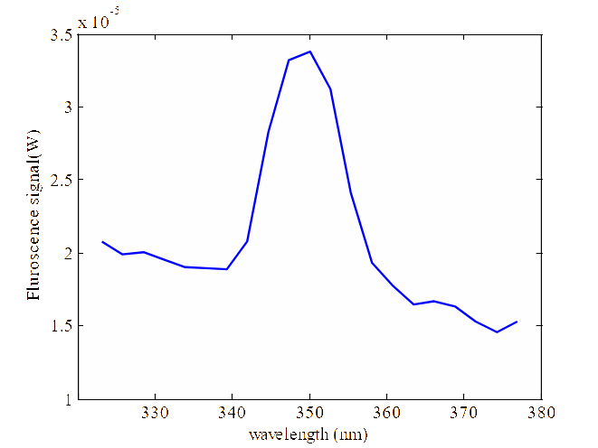
Figure 1 describes fluorescence spectra of the common fluorophors present in living cells after excitation with at 266 nm [13]. Due to differences in the constitution of the biological material of different particles, their fluorescence spectra are dissimilar. Standoff detection of biological agents is mainly based on the fluorescence from two molecules namely tryptophan and NADH. Tryptophan is believed to be primarily responsible for the fluorescence of bacterial agents. The intensity of the fluorescence signal from tryptophan is stronger compared to other fluorophors of the biological aerosols (see Figure 1). Hence, it is possible to detect the biological agents by using a suitable UV excitation wavelength. Currently, most prototype LIF LIDAR systems [14–16] use either 266 or 355 nm UV light; both these wavelengths being easily derived from a Nd:YAG laser, which has a small footprint, relatively low maintenance, and is readily available as a commercial source. 266 nm UV excites fluorescence primarily from the tryptophan within the bacterial cell wall and tyrosine (also NADH and flavins found in abundance in growth media) and 355 nm UV excites fluorescence primarily from NADH (and also flavins) but not from tryptophan. Therefore, it could be said that 266 nm light detects proteins present in the bacterial cell wall whereas 355 nm light detects compounds found in large quantities in growth media and which are less abundant in bacteria. However, the attenuation of 266 nm light by atmospheric ozone is approximately ten times greater than that of 355 nm and so 355 nm LIDAR systems may have a longer detection range.
![Fluorescence spectra of common fluorophors found in biological particles (spectra taken from [13]).](/journals/journal-of-battlefield-technology/volume-14/issue-02/assets/14-2-2-veerabuthiran/figures/figure01.png)
System description
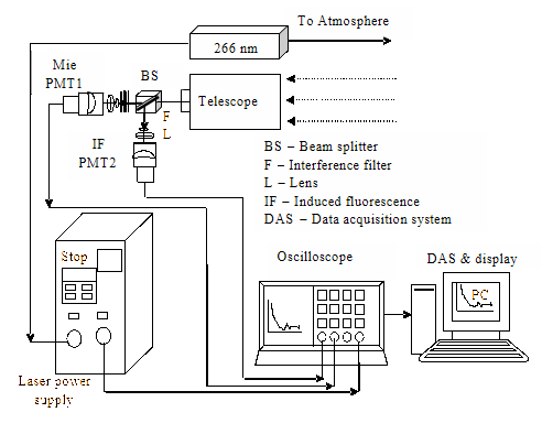
Figure 2 shows the schematic of the UV laser-induced fluorescence LIDAR (UVLIF) set up considered in this study. This system uses a Nd:YAG quadrupled wavelength of 266 nm as a source. A pulsed collimated laser beam is directed into the atmosphere towards the bioaerosol cloud. The divergence of the laser beam after collimation is approximately 0.2 mrad. The backscattered signal is collected using a Cassegrain telescope, which focuses the return signals onto the detector system which comprise a beam splitter, interference filter, lens and two photomultiplier tubes (PMT). A beam splitter divides the incoming backscattered signal and allows the radiation to reach the two PMTs. PMT1 is used to collect the elastic backscattered signals from the atmosphere at 266 nm whereas PMT2 collects induced florescence signals from the bioaerosol cloud. Two interference filters are used in this set up to block unwanted background light. PMT2 (fluorescence channel) is a time-gated detector and receives the return signal only if any bioaerosol cloud is present. The duration of the time gate (equal to the range of the cloud) is determined from the PMT1 (Mie channel) and the same information is fed to PMT2 to receive the signal from the cloud only. If the cloud is biological in nature then it will fluoresce at 350 nm due to the presence of tryptophan. The system will also determine the biological nature of the cloud by processing the signals received at both detectors. An interference filter with FWHM of 1 nm centred at 266 nm allows scattered signals to reach PMT1 and other filter with FWHM of 20 nm centred at 350 nm permits the induced fluorescence signal to reach PMT2. The detected signals are passed through an A/D converter and data processors etc. for signal analysis. A LIDAR master controller controls the laser transmitter, data acquisition and signal processing sequence in a photon counting mode.
Estimation of system parameters
Backscattered signals
The returned signal in terms of photon counting [17,18] at a range r is given by the following LIDAR equation:

where Ns is the number of received photons at the detector, Qd is the detector quantum efficiency; Et is the laser pulse energy (mJ); h is Planck’s constant; c is the velocity of light (m/s); λ is the laser wavelength (nm); A is the telescope area (m2); ηT is the laser transmitter efficiency; ηR the telescope receiver efficiency; φo the efficiency of the optical components; Δr the range resolution (m); βatm the atmospheric backscattering coefficient (m–1sr–1) due to aerosols and air molecules; βBA the backscattering coefficient due to bioaerosols (= Nbioσbio, where Nbio is the concentration of biological aerosols (ppl) and σbio is the fluorescence cross section of biological aerosols (m2)); r1 and r2 the bioaerosol cloud’s start and end range; αatm the atmospheric extinction coefficient due to aerosols and air molecules (= αa+αm) at the laser wavelength (m–1); αf is the extinction coefficient (m–1) at the fluorescing wavelengths (= Nbioρbio, where Nbio is the concentration of biological aerosols (ppl) and ρbio is the absorption cross section of biological aerosols (mm2/spores)); and NT is the total noise.
Detector Noise Limitation
The performance of the system is limited by noise from various sources. The received signal consists of optical background noise, the detector noise such as dark noise and Johnson amplifier noise. It is required that these noise levels should be quantified properly when estimating the system sensitivity. Total noise of the LIDAR signal is:
where Nb is the background noise counts, Nd is the dark current noise count, and Nampl the effective cathode amplifier noise count.
Background Noise
The background noise count received at the receiving detector is:
where Δλ is the optical bandwidth of the detection system (nm), Ωm is the receiving mirror field of view (Sr), Ar the area of receiver telescope (m2) and Lλ the spectral radiance of background source (Wm–2µm–1 sr–1) at λ. In general, the background intensity can be reduced by decreasing the receiver telescope field of view and optical bandwidth of the detection system. Since the system is being operated in the ultraviolet region, the background noise contributes significantly during daytime.
Johnson Amplifier Noise
Johnson noise is generated by thermal fluctuations in conducting materials. It results from the random motion of electrons in a conductor. The amplifier will add some equivalent noise photo-electrons, Nampl, to the effective cathode noise count, as given by the expressions:
where Δt is the detection interval (2Δr/c), Iampl the equivalent amplifier noise current at cathode (in amps), k is Boltzman’s constant (1.38×10⁻²³ JK–1), T the equivalent noise temperature of the amplifier, B the electrical detection bandwidth (7.5 MHz), M is the internal gain of PMT (106), and RL is a load resistance (50Ω).
Dark Noise
The dark current is the leakage current produced by the detector when there is no radiation falling on the surface. For the equivalent noise photoelectrons due to dark counts Nd, we have the expression:
A typical value for cathode dark current Id is 4×10–15 A. For a gain of 105, this implies Id = 8×10–17 A.
Measurement Sensitivity
The sensitivity of the system is characterized by the minimum concentration Nmin of the biological agent that can be detected with the minimum errors in optical signal. The expression for the minimum detectable concentration of biological agent is derived below under the condition of minimum signal-to-noise ratio (snrmin)—that is, ≥20. The signal-to-noise ratio (SNR) of the system for single pulse operation is:
where, Nampl is the Johnson amplifier noise, Nd the dark noise and Nb is the background noise. Adequate performance of the system requires snrmin ≥20. Averaging of multiple pulses is required to achieve this level. Assuming, we integrate over 1,000 pulses, the required single-pulse SNR would then be:
The required minimum number of detectable photons per pulse is determined using:
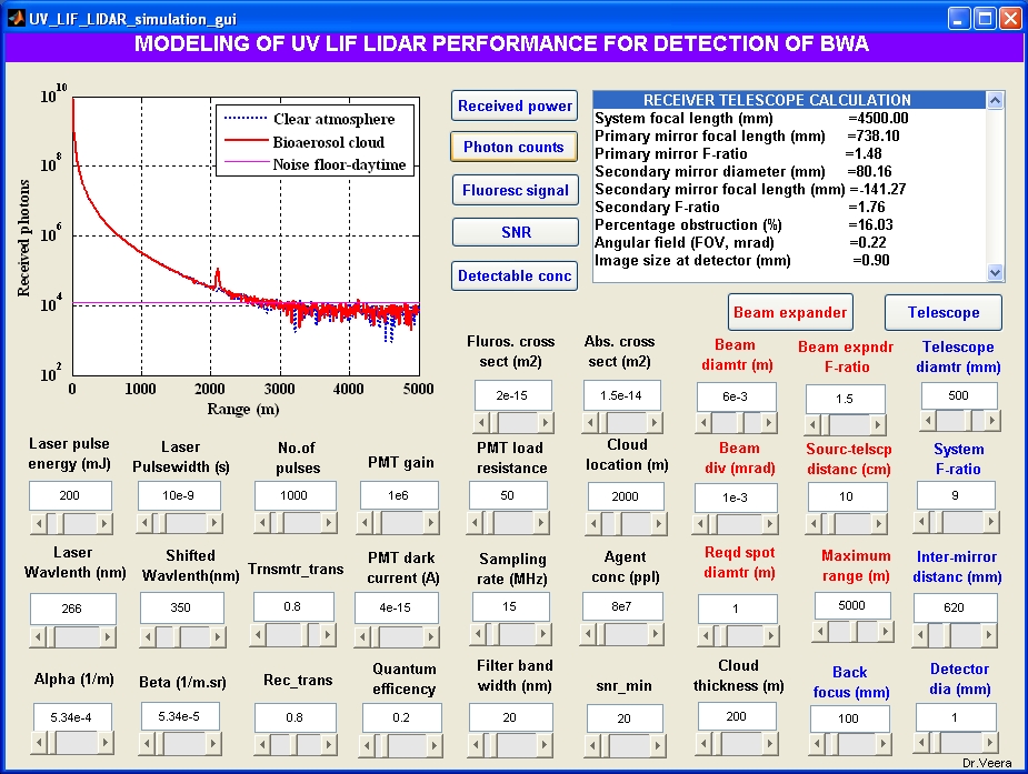
The values of Nb, Nd, and Nampl are determined as per the system specifications shown in the panel in Figure 3, and used in the above equation to obtain the minimum detectable photons. Once we know the minimum detectable photons per pulse, we can calculate the minimum detectable concentration of bioaerosols, (particles per m3) as a function of range, which is given by:
Discussion
Tryptophan is believed to be primarily responsible for the fluorescence of bacterial agents. It emits fluorescence signal, which peaks around 350 nm when it is excited by 266 nm UV radiation. The intensity of fluorescence signals from the tryptophan is stronger compared to other fluorophors of the biological aerosols. We aim to exploit this fluorescing property of tryptophan at an excitation wavelength of 266 nm for standoff detection of bioaerosol clouds. We present a LIDAR experimental setup, which receives elastic backscattered signal at one detector and a fluorescence signal at a second detector. We considered the scenario in which only the biological aerosols are released within the altitude region of 1 km or less in the atmosphere using any of the delivery modes available (such as UAV, aircraft, and artillery shells). After dispersal of the agent, it starts spreading due to background wind speed and forms stratified bioaerosol cloud layers. We have considered bacterial spores, bacillus globijii (BG)—a simulant of bacillus anthracis—of typical size 1 µm in our calculation. Depending on the spread conditions, they can agglomerate in clusters of sizes up to 10 μm. BG spores fluoresce at 350 nm when it is excited by laser radiation at 266 nm. The fluorescence cross section [19] of these bacterial spores at the fluorescing wavelength is 2×10–11 cm2/particles. We have not considered interferents such as road dust, diesel exhaust particulates, burning vegetation, and smoke in our calculation. The range profile of a simulated monodisperse of BG cloud of 200 m depth and peak concentration of 8×10⁷ ppl is assumed in our calculation, although the software program is general in nature and can cater for different values equally well. Aerosol concentration in the atmosphere is taken to be uniform. Further, we have taken the values for overall system efficiency (η) = 0.51 in our calculations (η = transmitter efficiency × efficiency of optical components × receiver efficiency). Using the above equations, we have determined the values of various parameters of the fluorescence LIDAR system for detection of BG spores. The present study aims to understand the various system parameters which influence the detection capability of this LIDAR. Figure 3 shows the graphical user interface (GUI) software developed in the MATLAB platform to perform the simulation studies. This GUI takes various input parameters of the laser source, receiver system, detector electronics parameters from the user and computes the return power levels, photon count, SNR, minimum detectable concentration, and so on, at various ranges. GUI has seven major push-buttons as shown in the panel in Figure 3. These buttons invoke various functions such as computation of return powers in terms of watts and photon count, SNR, minimum detectable concentration, etc. This program also computes the design parameters of a suitable beam expander for the laser source and receiver telescope. As an example, the return signal strength in terms of photon counts versus range for a BG cloud located at 2,000m is shown.
Initially, we have simulated the backscattered photon counts for clear atmospheric conditions using (1). The influence of βBA and αf is not considered in the calculation since no cloud is assumed. We have used system parameters such as Et=200 mJ, τ=10ns, PRF=20Hz, telescope diameter=500 mm and atmospheric parameters such as αatm = 5.0×10⁻⁴ m–1 and βatm = 1.09×10⁻⁴ m–1 at 266 nm in the calculation. Other input parameters are displayed in the panel in Figure 3. A similar curve is generated by introducing a bioaerosol cloud of thickness 200m and peak concentration of 8×10⁷ ppl between the distances of 2,000m and 2,200m. We used an absorption coefficient (αf) equal to 1.2×10⁻³ m–1 (=1.5×10⁻⁸ mm2/spores × 8×10⁷ ppl) in our calculation [20], which is typical for a 200m thick BG aerosol cloud. The background noise counts have been determined using (3) for the elastic and fluorescence detection channels by applying an appropriate bandwidth for the interference filters. Solar radiance values vary from 0.5–1 W/m2/nm for daytime operation. For night-time operation this value reduces to between 0.01 W/m2/nm and a negligible value. We considered solar radiance equal to 1 W/m2/nm for daytime operation and 0.01 W/m2/nm for night time operation in our calculation. The backscattered signals exhibit a peak between 2,000m and 2,200m, indicating the presence of the BG cloud at that range. It is seen clearly that return signals in the cloud region are stronger than the clear atmospheric signals, which is also higher than the noise floor level which is equal to twice the total noise counts. The simulated signals are meaningful only if they are higher than the noise floor. We have also introduced the white Gaussian noise in the simulated signal. Fluctuations in the return signal are high at the longer ranges, which indicates that the system cannot discriminate the cloud signal from the background noise level if it exists at long distances.
| Laser pulse energy (mJ) | Receiver telescope | Cloud type | Conc (ppl) | Maximum detectable range (m) | |||
|---|---|---|---|---|---|---|---|
| Diameter (mm) | F number | FOV (mrad) | Day time | Night time | |||
| 200 | 500 | 9 | 0.22 | 200 m thickness BG cloud | 8×10⁷ | 2,400 | 4,000 |
| 100 | 300 | 9 | 0.37 | 1,500 | 2,600 | ||
| 50 | 200 | 9 | 0.56 | 800 | 1,500 |
Similar performance studies have been carried out to select the best combination of system design parameters comprising the laser source and receiver telescope in order to develop a compact LIDAR set up. We have assumed three combinations namely: 1) pulse energy 200 mJ and telescope diameter 500 mm; 2) pulse energy 100 mJ and telescope diameter 300 mm; and 3) pulse energy 50 mJ and telescope diameter 200 mm. These combinations have been chosen based on their ready commercial availability. Figure 4 shows the backscattered signal as a function of range for the above combinations. LIDAR with any of the above three combinations can detect BG cloud at distance of ~700m. However, the LIDAR with pulse energy 200 mJ and 500 mm diameter telescope can detect the BG cloud maximum up to range of 2,000m in daytime, whereas the second combination can detect the cloud at ranges up to 1,500m.
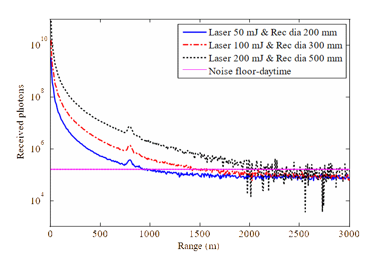
The maximum measurable distance is determined by moving the cloud location to different ranges by ensuring the cloud signals are stronger than the noise floor. Table 1 shows results of this analysis. For our research we aim to design and develop an easy to deploy and portable tripod mounted fluorescence LIDAR system, which can detect BG cloud maximum up to 1.5 km. A LIDAR with second combination would be the better choice to develop a compact and field deployable system.
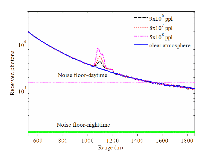
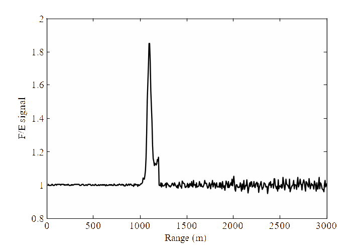
Critical analysis has been carried out for the LIDAR set up, which comprises a pulse energy of 100 mJ and receiver telescope diameter of 300 mm. Return signals have been simulated for transmission of a single laser pulse during day and night time operating conditions. Figure 5 illustrates the range dependent return signal at an excitation wavelength of 266 nm for a clear atmosphere, which decreases with range (solid curve in Figure 5). The return signals as a function of range are also simulated by introducing the bioaerosol cloud (dotted curve in Figure 5) using (1). The BG cloud of 200 m thickness is introduced between the ranges 1,000m and 1,200m with varying concentrations. The effect of βBA and αF due to the BG cloud is also incorporated into the calculation. Our analysis shows that this system can detect this cloud in daytime if its concentration varies from 9×10⁶ ppl to 5×10⁸ ppl. Figure 6 shows the simulated fluorescence signals received from the BG cloud located at distance of 1,000m. This signal is simulated for PMT2, which receives signals in the spectral band 350 nm ±10nm only if there is any induced fluorescence emitted from the BG cloud. A discrimination method is also being developed to evaluate the detection performance of the system. This method is based on the ratio of the fluorescence signal to the UV elastic signal for biological aerosols. Figure 7 shows the range profile of the ratio of fluorescence to elastic scattering signals. Strong enhancement in this ratio is observed in the bioaerosol cloud region, which confirms the fluorescence nature of the cloud. However, it is mentioned that the discrimination algorithms are based on the spectrally resolved fluorescence signature of biological aerosols and interferents (rather than the broadband fluorescence signal) and may result in improved discrimination performance.
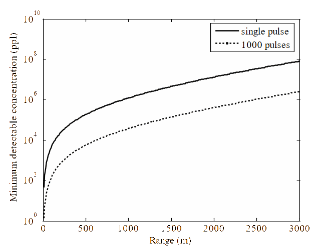
We have also estimated the sensitivity of the system in terms of minimum detectable concentration with respect to number of transmitted laser pulses. The minimum detectable BG concentration in particles per litre as a function of range for the minimum SNR) of 20 for transmission of single laser pulse and an average of 1,000 pulses were calculated and the results are presented in Figure 8. It is assumed that the averaging of multiple laser pulses improves the SNR by a factor equal to the square root of the number of pulses hence the sensitivity of the system increases significantly. The averaging of 1,000 pulses (equal to a detection time of 50 seconds) resulted in the fluorescence detection range of 520m for a lethal infective dose of ~10,000 ppl. Prior to the cloud dispersing to that concentration, it will have higher values. At 2,000m, it can detect the minimum concentration of 6.85×10⁵ ppl. The error in the fluorescence cross section values is expected to affect largely the determination of minimum detectable concentration.
Conclusion
We have presented the results of parametric studies of a fluorescence LIDAR set up to detect biological aerosol clouds in the atmosphere. We considered the fourth harmonics of a Nd:YAG laser operating (266nm) as a source and a Cassegrain telescope as a receiver with two detection channels namely: a Mie channel (elastic signal) and a fluorescence channel. The performances of various combinations of system design parameters have been determined and the system ability to detect a bioaerosol cloud located at 1–2 km during day and night time. We conclude, based on our studies, that fluorescence LIDAR with a pulse energy of 100 mJ and receiver telescope of 300 mm diameter would be the best combination to develop a compact and field deployable system. This can detect tryptophan contained a BG cloud of 200m thickness and concentration of 8×10⁷ ppl maximum at ranges up to 1.5 km during day time and 2.6 km during night time.
The sensitivity of the system is also evaluated in terms of minimum detectable concentration with respect to number of transmitted laser pulses. The minimum detectable concentration in particles per litre as a function of range for a SNR of 20 and for transmission of a single laser pulse and an average of 1,000 pulses have been determined. The averaging of 1,000 pulses (equal to a detection time of 50 seconds) resulted in a fluorescence detection range of 520m for a lethal infective dose of ~10,000 ppl.
References
J.A. Poupard, and L.A. Miller, “History of Biological Warfare: Catapults to Capsomeres”, Annals of the New York Academy of Sciences, vol. 666, 1992, pp. 9-20.
T.O. Toole, “Small Pox: An Attack Scenario”, Emerging Infectious Disease, Vol. 5, No. 4, 1999, pp. 540–546.
Potential military chemical/biological agents and compounds, January 2005 www.us.army.mil.
http://en.wikipedia.org/wiki/2001_anthrax_attacks.
http://news.bbc.co.uk/2/hi/uk_news/2636099.stm.
P.J. Wyatt, “Differential Light Scattering: a Physical Method for Identifying Living Bacterial Cells”, Applied Optics, Vol. 7, 1968, pp. 1879–1896.
C. Samuels, J.F.C. DeLucia, K.L. McNesby, and A.W. Miziolek, “Laser-induced Breakdown Spectroscopy of Bacterial Spores, Molds, Pollens, and Protein: Initial Studies of Discrimination Potential”, Applied Optics, Vol. 42, 2003, pp. 6205–6209.
S.E. Thompson, N.S. Foster, T.J. Johnson, N.B. Valentine, and J.E. Amonette, “Identification of Bacterial Spores Using Statistical Analysis of Fourier Transform Infrared Photoacoustic Spectroscopy Data”, Applied Spectroscopy, 57, 2003, pp. 893–899.
M.L. Laucks, G. Roll, G. Schweigers, and E.J. Davis, “Physical and Chemical (Raman) Characterization of Bioaerosols-Pollen,” Journal Aerosol Science, 31, 2000, pp. 307–319.
M. Manninen, A. Putkiranta, J. Rostedt, T. Saarela, M. Laurila, J. Marjamäki, Keskinen, and R. Hernberg, “Instrumentation for Measuring Fluorescence Cross Sections from Airborne Microsized Particles”, Applied Optics, 47, 2008, pp. 110–115.
P. Jonsson, F. Kullander, et al., “Development of a Fluorescence Based Point Detector for Biological Sensing”, Proceedings SPIE, Vol. 5617, 2004, pp. 134-142.
R.M. Measures, Laser Remote Sensing—Fundamentals and Applications, Kreiger Publishing Company, 1992.
S.C. Hill, R.G. Pinnick, S. Niles, Y.L. Pan, S. Holler, R.K. Chang, J. Bottiger, B.T. Chen, C.S. Orr, and G. Feather, “Real-Time Measurement of Fluorescence Spectra from Single Airborne Biological Particles”, Field Analytical Chemistry and Technology, 3, 1999, pp. 221–239.
S. Buteau, P. Lahaie, S. Rowsell, G. Rustad, K. Baxter, M. Castle, V. Foot, R. Vanderbeek and R. Warren, “Laser Based Stand-Off Detection of Biological Agents,” NATO Report RTO-TR-SET-098 (2009).
J.R. Simard, G. Roy, P. Mathieu, V. Larochelle, J. McFee, and J. Ho, “Standoff Sensing of Bioaerosols using Intensified Range Gated Spectral Analysis of Laser Induced Fluorescence”, IEE Transactions on Geoscience and Remote Sensing, 42, No. 4, 2004, pp. 865–874.
K. Baxter, M. Castle, S. Barrington, P. Withers, V. Foot, A. Pickering, and N. Felton, “UK Small Scale UVLIF LIDAR for Standoff BW Detection”, Proceedings of SPIE, Vol. 6739, 2007, pp. 67390Z-1–67390Z-10.
O. Steinvall, P. Jonsson, and F. Kullander, “Performance Analysis for a Standoff Biological Warfare Agent Detection LIDAR”, Proceedings of SPIE, Vol. 6739, 2007, pp. 673912-1 to 673912-14.
D. C. Steven, C.N. Meltow, M.S. Desha. A. Wong. M.W. Wilson and J. Butler, “UV Fluorescence LIDAR Detection of Bioaerosols”, Proceedings of SPIE, Vol. 2222, 1994, pp. 228–237.
V. Sivaprakasam, A. L. C. Scotto and J. D. Eversole, “Multiple UV Wavelength Excitation and Fluorescence of Bioaerosols”, Optics Express, 12, 2004, pp. 4457–4466.
J. Kunnil, S. Sarasanandarajah, E. Chacko, and L. Reinisch, “Fluorescence Quantum Efficiency of Dry Bacillus Globijii Spores”, Optics Express, 13, 2005, pp. 8969–8979.