A Computational Approach To Situational Awareness: A Follow-Up On The Details

I. introduction

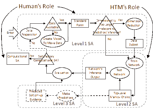
The aim of this paper is to create a computational situational awareness (SA) usable by the Department of Defense to gauge Iraq’s stability during 2003–2008. This SA applies to the Iraq War from 2003–2008, which henceforth will be called the ‘Iraq context’. To do so, we will implement a method that is summarized by the information flow of Figure 1. This method maps the machine learning algorithms to be used here (Hierarchical Temporal Memory, or HTM) [1],[2] to the three levels of SA first hypothesized by Endsley [3]–[5] and subsequently accepted by other human factors researchers. These three levels are Level 1 (perception of relevant elements), Level 2 (comprehension of those elements) and Level 3 (prediction). Here, we focus on Levels 1 and 2, since they are a necessary antecedent to Level 3. In particular, we present here a way to implement Levels 1 and 2 for this problem via data pre-processing and HTM training/testing.

While this approach enhances awareness of trends in the data of the Iraq context, it also mimics the basic tenets of what constitutes SA in actual decision-makers. In particular, Endsley and others have shown that the selection of a goal is crucial to SA formation. Here, we assume the criteria for success established by the U.S. Department of Defense: to bring Iraq to political, economic and social stability between 2003–2008 [24]. Consequently, we rely on data related to these aspects of the Iraq context, so that not only do we enhance a decision-maker’s own SA of the Iraq context but we also create one—albeit, a rudimentary one—with a computer.

To account properly for the complexity of the Iraq context, our method must be carefully applied. Specifically, SA of this context is not easily validated, since we do not know the ‘right answer’ a priori. Although this is possible in other learning problems, such as invariant visual pattern recognition, we cannot do this here. So to verify the accuracy of the computational SA formed in this context, a new method will be introduced that has influence from system dynamics: we call it extreme-case bounding. This method has assumptions built into it that creates fictitious extreme cases of stability, either extremely unstable or extremely stable. With these fictitious bounds used for HTM network training/testing, some insight into the actual progression of events in Iraq during 2003–2008 can be obtained. Needless to say, this method is not perfect and it is somewhat arbitrary because we arbitrarily select a peg against which to measure Iraq’s stability. Nevertheless, it provides an intriguing foothold in an avenue of computational SA that has thus far been difficult to probe concretely. For instance, in previous work on this subject [6], it was only possible to grade the computational SA against qualitative reports. We propose extreme-case bounding as a quantitative alternative, or at least a complement, to that approach.

Throughout this paper, we follow the information flow of Figure 1. Entering the flow from the top-left yellow arrow, we first accomplish Level 1 SA (that is, perception of relevant elements). In the course of doing so, we will see that the availability of data is both true and false. It is true in the sense that we actually have real data on the context we wish to understand. But it is false in the sense that we must model extreme-cases to provide boundaries to this real data. Thus, some modelling will be needed to generate that additional data. The data will then be put into an acceptable format for analysis before training and testing with HTM networks. Though not discussed thoroughly here, there was only minimal iteration between data generation and network training/testing. In this paper, we will train HTM networks on extreme-case data and test them on actual data. Afterwards, we will make conclusions about the resulting Level 2 SA (that is, comprehension) on the Iraq context. As we have mentioned, the evaluation will be a little more difficult, but the focus on extreme-case bounding will help in this regard. Furthermore, we will see that extreme-case bounding is a more substantive approach than the qualitative comparative analysis offered by an earlier paper on this exact problem [6].

This introduction (Part I) has laid out the approach to computational SA discussed in this paper. Part II will detail how the real data is prepared for analysis with an HTM-based SA. Part III will then describe how the extreme-cases are generated. Part IV will be the real focus of this paper: in this section we will build and test various implementations of computational SA for the Iraq context. In Part V, we will briefly compare the method and results of Part IV with a qualitative comparison to the SA described in DoD reports. Part VI will then allow us to draw conclusions.

Ii. level 1 sa: data preparation

Entering the information flow of Figure 1, the first task (represented by an oval) is to prepare the data. Before doing so, we must address the Boolean question (represented by a triangle) about whether data is available. For the Iraq context, we actually have data. But some effort is needed to prepare this data into standard form.

There are four issues we must confront in doing so. First, the primary source [7]–[18],[19] from which the data is extracted contains many blanks in the data, depending on how many metrics are used. So a set of metrics must be selected from the actual data that exhibits a minimal number of blanks.

Second, the primary source has not prepared the data in a temporally structured format suitable for HTM learning. Dileep George pioneered work on HTM algorithms and he gives guidelines for generalizing their usage in other domains. In particular, George writes, “if there is no temporal structure in the data, application of an HTM to that data need not give any generalization advantage.” So the data must be arranged in this fashion if HTM is to be of use. Specifically, observations at specific time intervals should follow one another.

Third, the relative magnitudes of the chosen metrics will be necessary to consider. Consequently, a transformation of the data may be necessary before training/testing.

Fourth and finally, one of the metrics we use to describe the Iraq context is only known within given bounds at each time step. Consequently, we must select a technique to get only one value at each time step, rather than a range.

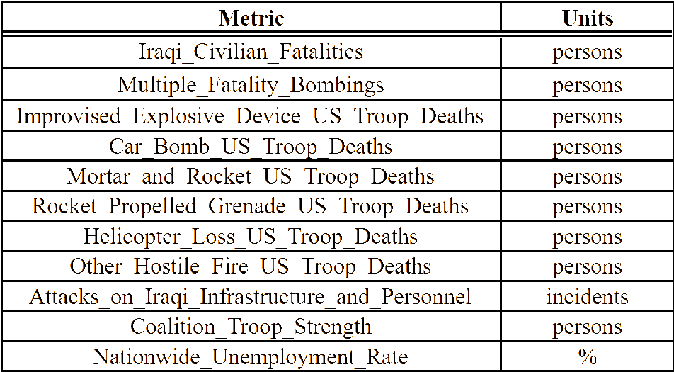
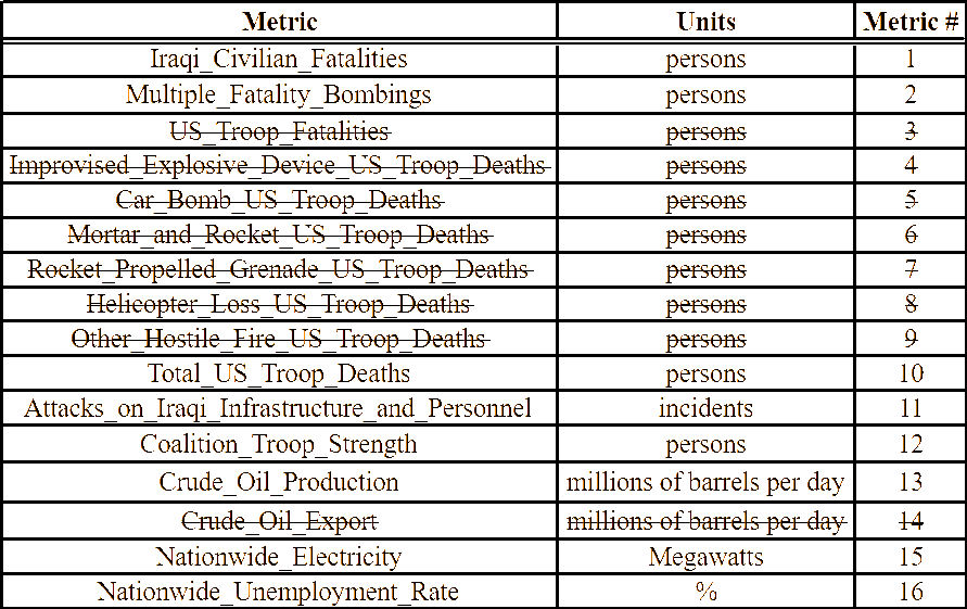
So we cautiously probe each of these steps with more detail now to prepare the data in standard form. Due to the need for minimally blanked and temporally sequenced data, only a set of sixteen metrics whose values change monthly can be used. These metrics are shown in Table 1 with identifying numbers next to each of them.

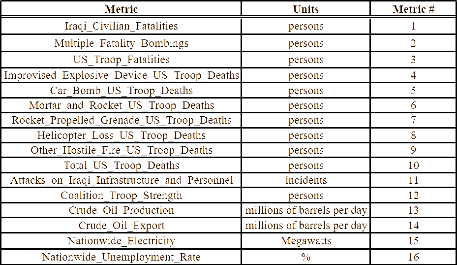
While it is possible to select fewer metrics, a drop off in performance was seen when this was done [20]. We will show this in a later section. We believe that this occurs because the degree of stability in an operational theater already lacks a clear definition amongst stakeholders. Consequently, the more metrics that are incorporated into the analysis, the more complete the description of stability will be. Here, we stopped at sixteen because of what was publically available, but more metrics may make the analysis that much more rich.

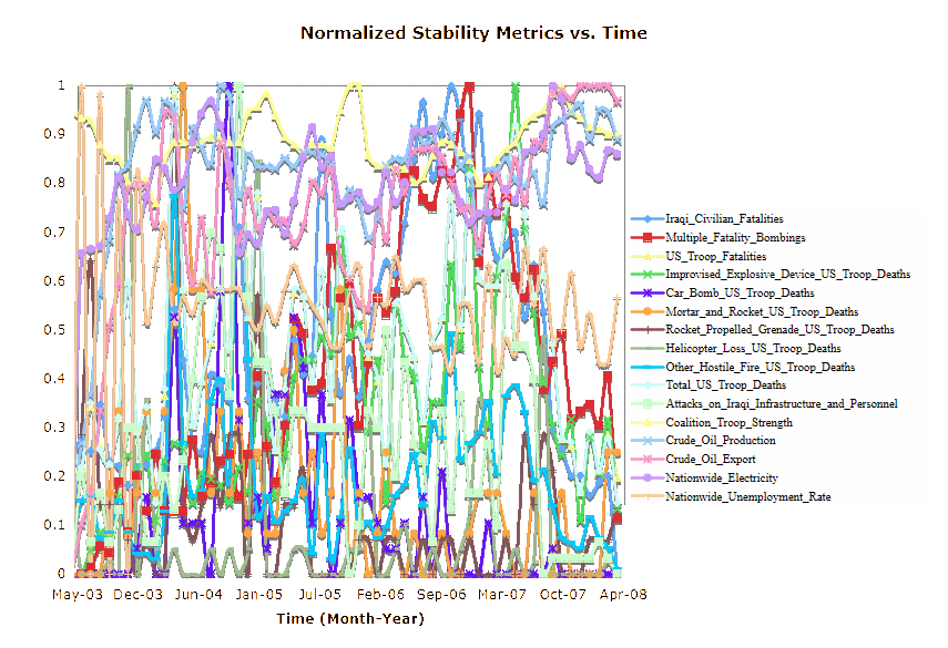
Most of the metrics shown in Table 1 are known monthly from May 2003 to April 2008 [19]. Still some of these metrics are only known as ranges of values. But for the purpose of analysis with HTM, it is necessary for these metrics to have single values too. Therefore, with regards to the fourth issue raised above, a random number within that range has been chosen each month. This is done rather than choosing the midpoint because the same range was seen over multiple months. Consequently, a random value chosen from a uniform distribution would preserve some of the uncertainty in this metric’s value. Finally, addressing the third issue of relative magnitudes, all metrics are normalized by their maximum value recorded between May 2003 and April 2008. This gives us the convoluted plot shown in Figure 2, in which all sixteen metrics are shown. It should be quite clear from this plot that at any given month it is not a simple problem to infer the stability or lack thereof in Iraq. But this is in fact the aim of a computational SA of the Iraq context. To aid our creation of this SA, we assume that heuristic extreme-cases of instability and stability can provide a bound on the reality shown in Figure 2. These extreme-case scenarios are assumed to develop from a real data point and then to evolve in time. This ensures that the HTM learns a progression of events leading towards our arbitrarily decided states of stability and instability. So we turn our attention there in the next section.

Iii. more level 1 sa: extreme-case bounding

Now that the actual data has been prepared in a format that is suitable for HTM generalization, we face another difficulty. As noted above, we do not know exactly how to validate the HTM output. There is no visual basis for validation as there would be, for instance, with using HTM for invariant visual pattern recognition [1,2]. In short, there is no simple way to determine a stable situation from an unstable one, either by natural human information processing or a closed set of consistent equations. So our method for validating HTM categorization output will rely on the predefined goal of bringing stability to Iraq.

The method for validation that is proposed and done here is called extreme-case bounding. In light of no alternatives, this bounding is an arbitrary estimate on a stability reference frame. This method uses artificial data that represents Iraq’s stability becoming increasingly worse or better from an actual data point (here, April 2008 was used). It is then speculated that reality exists between these bounds. Consequently, we should be able to get a measure of how close or far a given month is to these progressions to stability/instability. A one-dimensional representation of this concept is shown in Figure 3.

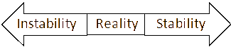
But in the context of Iraq, the dimensionality will be higher than Figure 3 shows. Instead, there will be extreme-cases for each of the sixteen dimensions by which stability is measured. To analyse this claim some tests are done and results are shown in subsequent sections. But first, it is important to specify the system dynamics model that will generate this extreme-case data.

The goal in creating such a model is to generate data that is either clearly asymptotically stable or unstable. For simplicity, we assume that stability is a monotonic function of each metric. For instance, a smaller number of U.S. troop fatalities is linked to greater stability. Although more sophisticated models have been proposed [23], let us simplify things even more by making all metrics either linearly increase or decrease. We will note a distinction with other insurgency models (in particular, that of Bohorquez et al. for casualties) in a discussion to follow. In system dynamics terminology [21], the factors affecting the Iraq context will linearly change the values of context metrics every time step (here, this is one month). It is assumed that a five percent change in the value each time step is done, for both unstable and stable cases. This linear change is chosen to generate changes in the metric values that do not saturate too quickly. This allows the HTM to learn during training how a real data point can progress to stability/instability. As an exception, nationwide unemployment is slightly altered in the stable case so that the value does not drop too fast. This is implemented directly in an Excel spreadsheet. In doing so, it is important to follow certain guidelines on system dynamics modelling, such as conservation laws between metrics (Table 2) and boundaries on certain metrics (Table 3). In short, these boundaries and conservation laws are followed because first-order system dynamics models can exhibit exponential behaviour [21].

It should be noted that the conservation laws of Table 3 are assumed here, but for good reason. First, the equality of U.S. Troop Fatalities and Total U.S. Troop Deaths is done because in the real data of 2003–2008 there are at least two discrepancies in these metric values. This happened because the monthly measurements did not occur on the same day. For our extreme-case model however, we ignore this sampling error and hence equate the two values. Second, the number of Total U.S. Troop Deaths (equated to U.S. Troop Fatalities) must be equal to the number of specific ways U.S. troops died (such as from car bombs, helicopter crash, and miscellaneous).

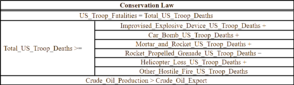
The ‘greater than’ is used to reflect the miscellaneous deaths not explicitly contained in the sixteen metrics used here. Finally, we assume that Iraq does not export all of its crude oil, and so require that exports do not exceed production.

But why should there be boundaries on some of the metrics? For instance, Bohorquez et al. have shown that the frequency of causalities in human insurgency obeys a power law relationship to the number of casualties [23]. But these power laws are somewhat different because they apply to event size (independent variable) and frequency (dependent variable). In particular, for Iraq 2003–2008, they found that the frequency (p) evolves as x^–a, where x is the number of casualties and a ~ 2.35. Since we are explicitly modelling temporal dynamics, we must work with event size as the dependent variable and time as the independent variable. Consequently, such power laws do not affect our choice to bound these variables. If anything, such laws could add higher fidelity to the way that the number of casualties evolves in time. For our implementation, we have assumed a linear approximation to the evolution of this metric in time.

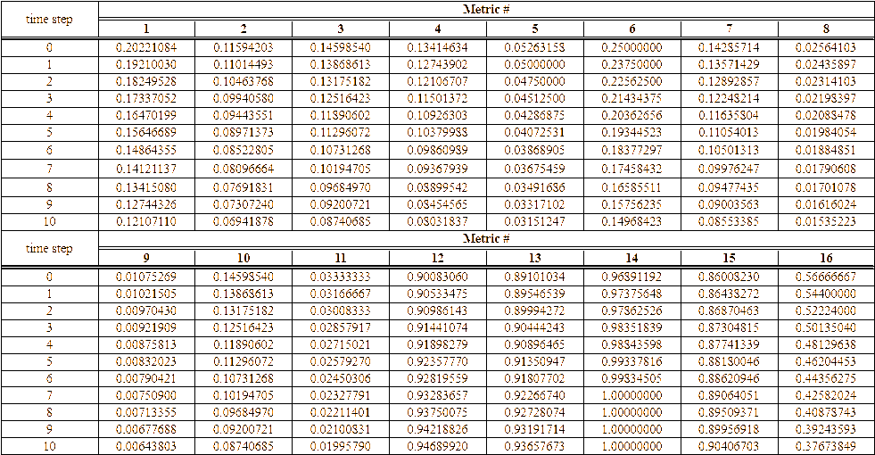
Starting from an initial condition, we generate progressions towards extreme stability and instability, as determined by our assumptions of conservation (for example, Table 2), bounding (for example, Table 3) and linear evolution. An excerpt of this dataset is in Table 4. Notice that metrics inversely changing with stability, such as Iraqi Civilian Fatalities (metric #1) and U.S. Troop Fatalities (metric #3), decrease with time for monotonically stable contexts.

Conversely, metrics that increase with stability, such as Crude Oil Production (metric #13) and Nationwide Electricity (metric #15), increase with time. It is important to emphasize that this is not a model for the reality of how the Iraq context evolved. Rather, this is a model for the ways that extreme-cases of Iraq stability/instability can be reached. This model is important because it provides heuristic boundaries to the reality. These boundaries are important for training the HTM. For ease of reference, we will call these extreme-cases the ‘monotonic extreme-cases’. With this new data, let us turn now to analysis of HTM-based Level 2 SA.

Iv. building and testing computational sa

With the ability to generate data for both progressively stable and unstable situations, as well as the actual time series of data on the Iraq context, it is possible to attempt HTM as an unsupervised machine learning mechanism. In short, an HTM is a network trained with K-means clustering and then used to perform evidence-based Bayesian inference on novel data [1–2]. With HTM, the aim now is to fuse the data and to extract possibly implicit meaning from it. We emphasize the unsupervised nature of the learning here because our goal is to extract implicit meaning and not to impose our possibly biased judgments. Furthermore, we attempt to extract this meaning from a system that is not ergodic (that is, there is no end-state), not separable into components and not completely observable. So we employ now a two-pronged approach to the training and analysis of these HTM networks. The first is to use actual data and the second is to use extreme-case data. But a question arises as to how the data should be used. Should the HTM be trained with the real data and tested on the extreme-case data? Or, should it be trained with the extreme-cases and be tested on the actual data? Here, we will implement the latter ordering so that the HTM can learn from the extreme-case boundaries and then use them to classify the reality in between.

The evaluation of this computational SA is not entirely straightforward. Consequently, some additional techniques are employed here to probe the SA formed about the Iraq context. For instance, we do not know if too many or too few metrics are being used here to describe the Iraq context. So we will see what the effects on training/inference are when the number of metrics is reduced from N = 16. Also, we will examine the degree to which information is hierarchically stored in intermediate levels of the networks. Finally, we will consider alternative ways of feeding the data into the networks to see what effects—if any—there are on the simulated SA.

Why would we use these techniques in particular? For instance, what purpose could there be in probing the hierarchical storage of information in an HTM? It is necessary to recall that our purpose in using HTM for computational SA has been its declared ability to condense information into hierarchies of both space and time. For the Iraq context, we test hierarchical storage directly because it is not clear what the top-level node’s output should be, as it might for simpler recognition tasks (such as invariant visual pattern recognition [1]). One possible outcome of this analysis is that it might in turn help us to identify what aspects of the Iraq context are not well observed. This would then provide the beginnings of a feedback mechanism with Level 1 SA to search for more data. In fact, in the course of this research, it was one possible feedback mechanism between Levels 1 & 2 SA that informed us to improve our extreme-case model. This resulted in the monotonic extreme-case models. Necessarily, this is not the only possible feedback mechanism, but as we will see, it helps to strengthen the credibility of the Level 2 SA formed here computationally.

Finally, there is one other tool at our disposal that has not been mentioned. Specifically, we could use the DoD reports on stability in Iraq [7]–[18] in a comparative analysis. In fact, such a comparison was the aim of a previous paper [6]. But as we will see, the use of extreme-case bounding provides more concrete analysis than such comparisons. We now turn to our experiments and their analysis.

Since we use data that is monotonically extreme, we expect an HTM network to learn to recognize clear progressions towards stability/instability. We employ an evolutionary approach to network design here and modify a network used in an HTM demonstration example (see Waves in [22]). In order to exploit the HTM network’s temporal learning algorithms, we modify the network parameters to accommodate how the metrics’ values change in time. The complete network parameters employed for this computational Level 2 SA can be seen in another work (see appendix C.9 in [20]). After training the network, we see that there are sixty-one coincidence patterns (C^3,1) and fifty-nine Markov-chains (G^3,1) in the top-level node. The coincidence patterns are the result of the K-means clustering in this top-level node, while the Markov-chains are the result of first-order transition probabilities between these coincidence patterns. This is a standard calculation for each of the nodes in an HTM network (see George [1] for more details). But the real point of training an HTM network is to see its inference performance. We will start plaintively by looking at inference on the training data.

When we perform inference on training data, we see a clear progression of Markov-chains as instability increases, but stability is still not clear. We can see this by following the probability over Markov-chains ${\lambda }_t\left(g_r\right)$ of the top-level node, given the bottom-up evidence (^–e_t) at each t. In particular, we examine the maximum of this distribution ($\text{max}\left[{\lambda }_t\left(g_r\right)\right]$) to see what stability state is most likely. A complete history of the top-level node feed-forward inference can be found in another work (see appendix C.19 of [20]). First, let us examine the inference output during what we know from the data to be a progression towards instability. We see that each of the Markov-chains is distinct for each time step. The progression indicated by $\text{max}\left[{\lambda }_t\left(g_r\right)\right]$ is g0, g1, g2, ..., g58. Since we know the data is monotonic towards instability, we can reasonably claim that the Markov-chain labels are monotonic towards instability as well. For example, the bottom-up evidence when g45 is most likely in the top level indicates a situation that is less stable than when g5 is most likely.

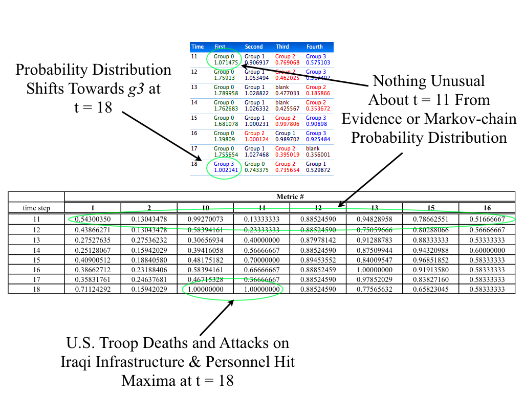
Having trained the network to recognize progressions in instability, it would be useful now to test this ability on real data of the Iraq context. When we look for instability gradations in the actual data, we see some interesting results (Figure 4). In Figure 4, as in similar figures to follow, each row is a time point. The first, second, third, etc. columns indicate the groups (Markov-chains) that are most likely, second most likely, third most likely, and so on, given the bottom-up evidence. The significance of this ordering of group numbers at each time point is that we can quantitatively say how unstable Iraq is at each of them. Note throughout that time points t ∈ [0,60] correspond to each month from May 2003 to April 2008. In particular, at t = 11,12, the entire probability distribution over top-level Markov-chains shifts towards higher number Markov-chains. At t = 11, g25, g24, g23 are in the top three (see Figure 4).

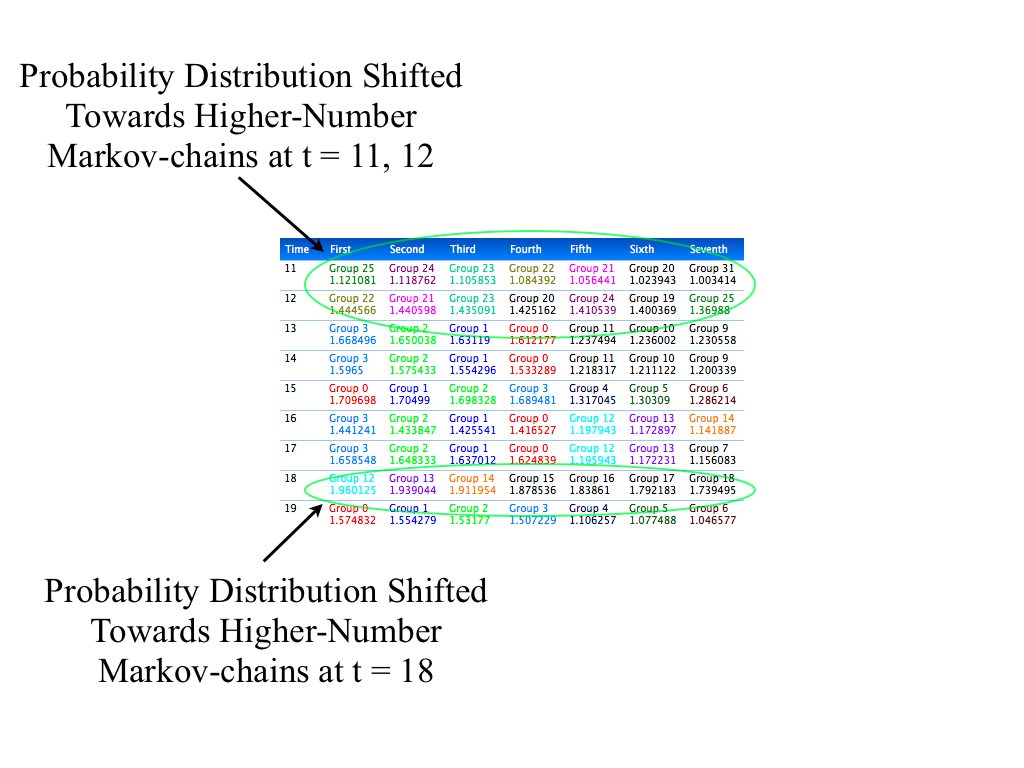
At t = 18, the probability distribution shifts as well, indicating g12, g13, g14 in the top three. In light of our results from inference on the monotonic-extreme-case instability data, it would seem that the Iraq context is increasingly unstable during these months. Furthermore, the actual data during these months indicates this in comparison to those months that come before them.

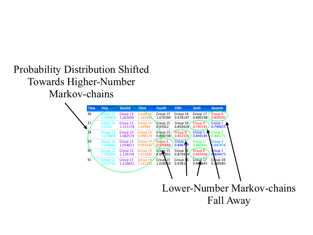
Let us expand our purview to those time points leading up to and coming out of t ∈ [41,49], another region of heightened instability according to the network. If we consider the top seven Markov-chains of the top-level for t ∈ [36,60] then we see something quite interesting. For t ∈ [36,41], the distribution shifts increasingly towards g12, g13, g14, g15, g16, g17, g18. We can see this by the demotion of g0 over these time steps too (Figure 5).

Then for t ∈ [41,49], these seven Markov-chains are the most likely, given the bottom-up evidence (Figure 6).

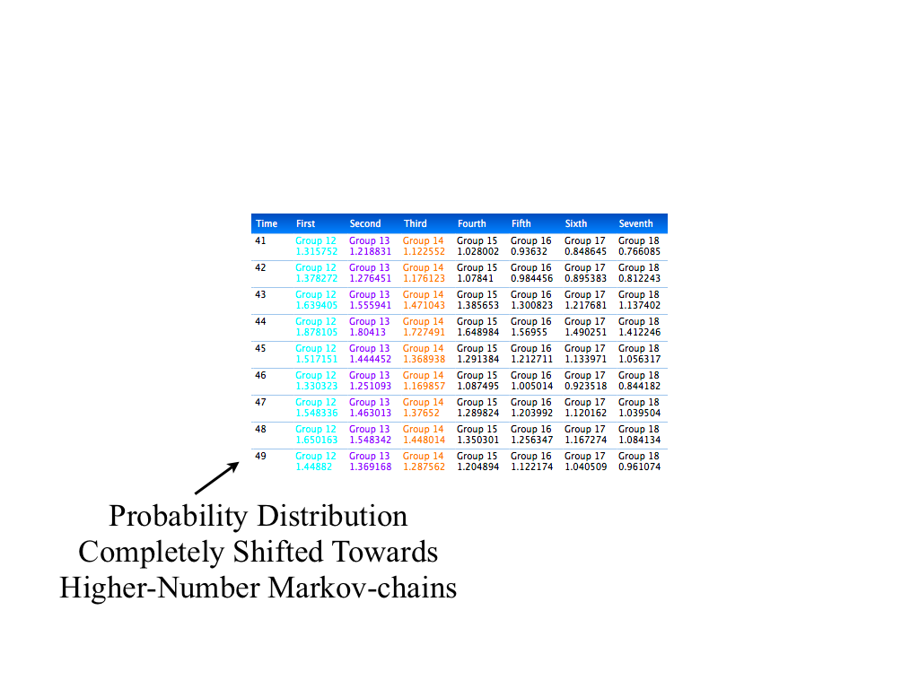
As we know from the actual data, there were peaks in violence and other attacks, sagging economic metrics, etc. during this time. But there were also metric trends that favoured stability. Consequently, this conflicting data makes it difficult to characterize the stability level during this time period. But here we see the probability distribution shift for the entire time period towards these mid-grade instable states.

The situation in the Iraq context changes with time. For t ∈ [50,51], the probability distribution begins to shift back. Finally, for t ∈ [52,60], g0, g1, g2, g3 are the top four most likely Markov-chains (see Figure 7).

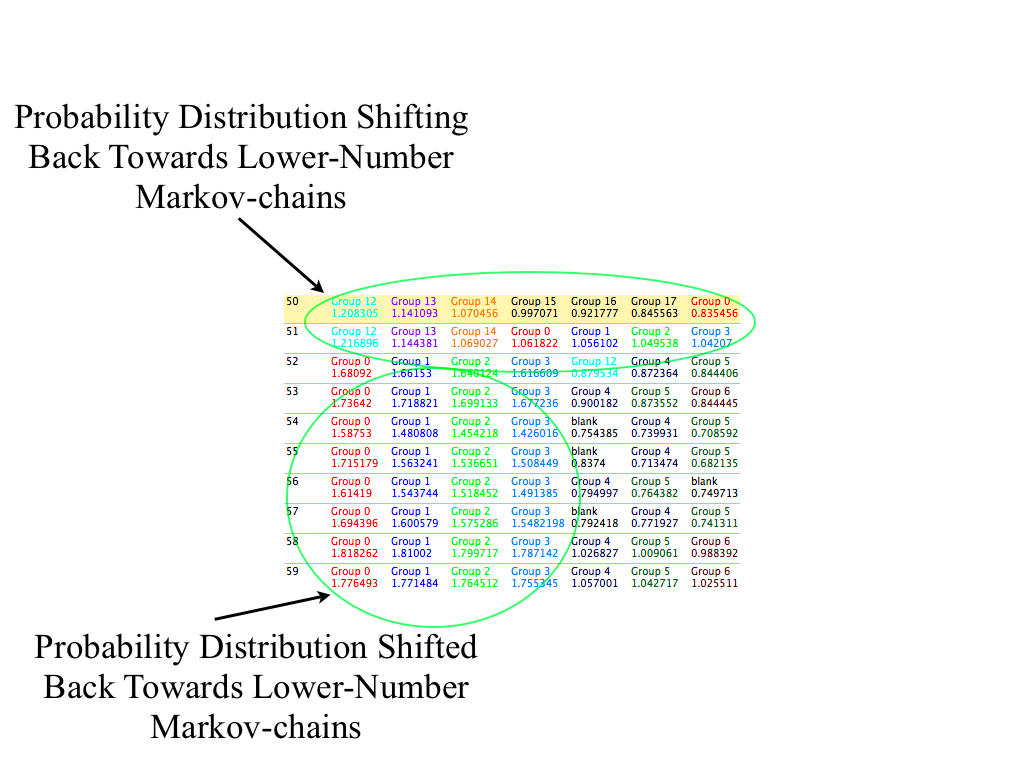
Even though this does not indicate stability, it does indicate a dramatic drop in instability, according to how we trained the network. So we see here how the monotonic training data has provided a peg against which to categorize evidence that trends towards instability. But what about stability recognition?

As mentioned earlier, direct stability recognition is less clear, even with the monotonic training data. Rather, we can only infer stability recognition with the network. Why is this so? If we consider the types of metrics used here then we notice that only four of them increase with stability. So, as a more stable situation is reached, the remaining twelve metrics drop close to zero. Consequently, the bottom-up evidence does not provide enough magnitude to propagate through the network. All the change comes from the four metrics that increase with stability. In the current permutation of the data, one of them is in the receptive field of the third node in level one (N^1,3) and the other four are in the field of N^1,4. The entire left receptive field (covered by N^1,1 and N^1,2) therefore produces blank recognition. This is because there is simply not enough bottom-up evidence coming up through this side of the network. So we are not able to determine gradations of stability because the utility function of these metrics can be assumed to be inversely proportional to stability. Consequently, as stability is reached, the magnitude of ^–e_t goes to zero. In future implementations, it might be possible to alleviate this problem by transforming the data by an inverse or offsetting the zero. We have not done this, however, because we have devised an approach to recognize degrees of instability in real data, as judged against the extreme-case baseline. Furthermore, these results imply stability recognition due to the monotonic utility function of stability/instability.

As stated earlier, we employ some additional tests to examine the results in more detail and we now recall those techniques. We shall examine: whether fewer metrics can be used to produce similar results; how results change if the data is fed in differently; and, to what extent information is stored hierarchically. We will begin with an analysis of the effects from reducing the number of metrics.

We first reduce the number of metrics from N = 16 to N = 8. We will then train and test the HTM network on the Iraq context via these metrics. We will see that there is slight degradation in top-level inference performance as the number of metrics is reduced.

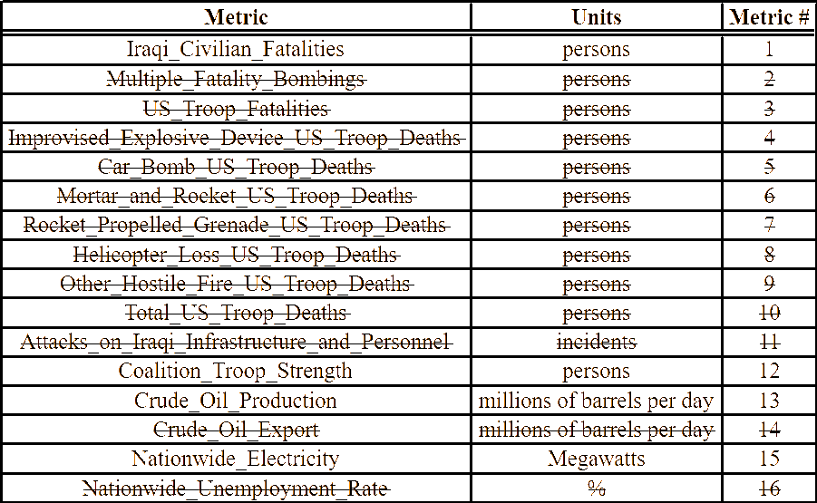
We begin by reducing the dimensionality of the input vector space from N = 16 to N = 8. The original N = 16 dataset is rich on data pertaining to various ways that U.S. troops were killed in combat, such as deaths related to RPGs, helicopters and other hostile fire. Now, we wrap all of this data into the total number of U.S. troop deaths. Also, we no longer have redundant data on the number of U.S. troop deaths, as we had earlier with U.S. troop fatalities. We keep three out of four politico-economic metrics, eliminating only crude oil export, which is dependent on crude oil production. The final metrics for the N = 8 input vector space are shown in Table 5. The ones that have been omitted are also indicated. All of the original metric numbers are kept for ease of continuity with previous work.

After training on monotonic extreme-case data, the top-level node learns eight coincidence patterns (C^3,1) and four Markov-chains (G^3,1). When we look at inference on the training data, we see similar results to what we have seen earlier. The complete inference history is shown in another work (see appendix C.21 of [20]). In particular, the monotonically stable states drive to zero and so produce blank Markov-chains that propagate up through the network. Also, the monotonic sequence of Markov-chains from $\text{max}\left[{\lambda }_t\left(g_r\right)\right]$ reflects the monotonicity in the unstable training data. Specifically, this network recognizes the following sequence of Markov-chains via $\text{max}\left[{\lambda }_t\left(g_r\right)\right]$: g0, g1, g2, g3.

When we perform inference on actual data, we see some interesting similarities to the N = 16 case. For instance, at t = 18, g3 is the most likely Markov-chain of the top-level node. In other words, there is a higher state of instability at t = 18 than there was at surrounding time steps. This is what happened in the previous network, which was trained on N = 16. But it does not recognize anything in particular about t ∈ [11,12]. If we consider t = 11, it seems that this occurs because the evidence was stronger at t = 18 (see Table 6).

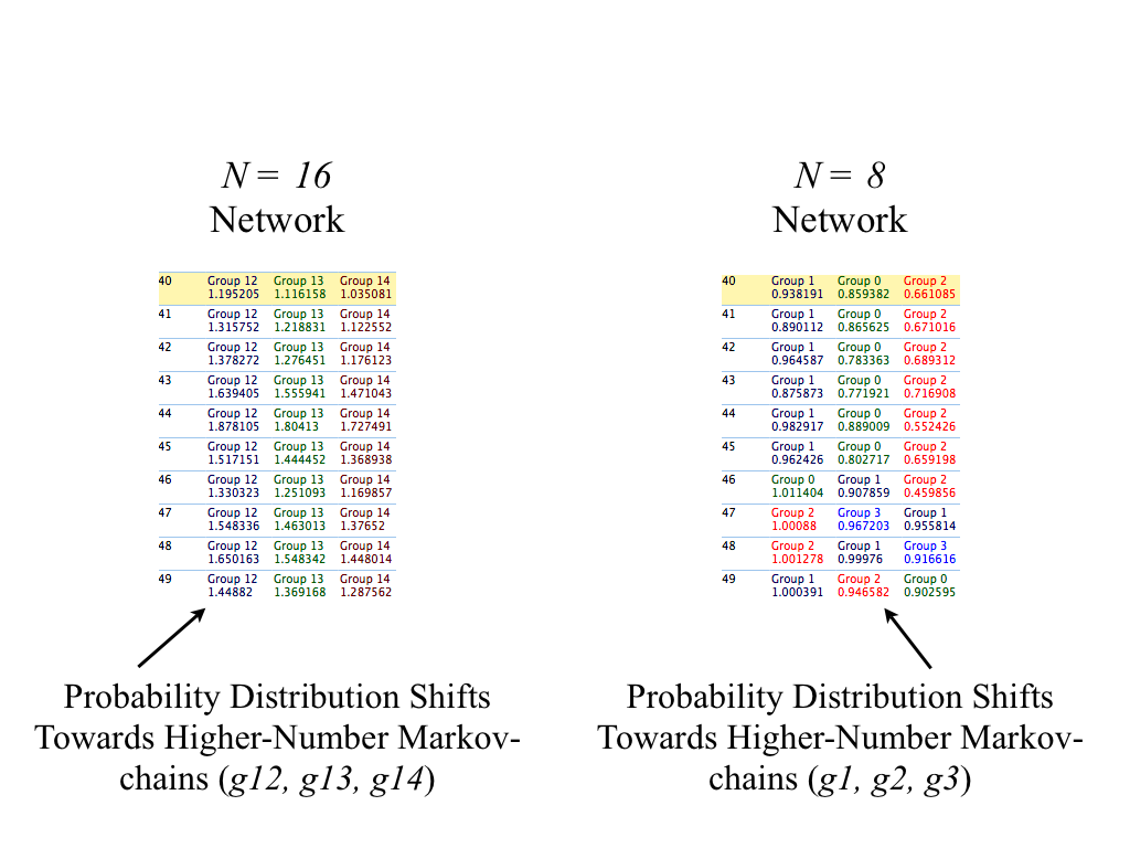
For instance, as the table shows, both U.S. troop deaths and attacks on Iraqi infrastructure/personnel hit a maximum at t = 18. The same reasoning applies to t = 12 in relation to t = 18 too. Also, for t ∈ [40,49], we see some interesting results that are similar to what has been seen before for N = 16. For t ∈ [40,45], $\text{max}\left[{\lambda }_t\left(g_r\right)\right]$ indicates g1. Then for t ∈ [47,49], we see $\text{max}\left[{\lambda }_t\left(g_r\right)\right]$ indicates g2 and g1. So this indicates, as before, that these time points have evidence indicating instability. This is similar to what was seen for the N = 16 network trained this way (see Figure 8).

So we see that when we reduce the number of metrics, the recognition of “unstable” states is maintained when looking at the actual data. What about when we reduce the number of metrics further?

We reduce the number of metrics to N = 4 and assess training/inference results, having trained on the monotonic extreme-cases. For instance, we can keep only Iraqi civilian fatalities, coalition troop strength, crude oil production, and nationwide electricity (see Table 7). These metrics provide a rough account of security, politico-economic conditions and surge effectiveness.

Turning to training of the HTM network, the top-level node learned four coincidence patterns (C^3,1) and three Markov-chains (G^3,1). When we look at the inference on the monotonic training data, we see encouraging results. The complete inference history can be found in another work’s appendix (see C.22 of [20]). For instance, the monotonicity of groups indicated by $\text{max}\left[{\lambda }_t\left(g_r\right)\right]$ is seen during stable states. We see that g1 follows g0 as the states become more stable. Also, the top-level node indicates a monotonic progression of Markov-chains for unstable states: g2 follows g0. But when looking at inference on the real data, the results are inconclusive. So it seems that we have hit a threshold. In other words, when the number of metrics is reduced below some threshold between N = 4 and N = 8 metrics, there is simply not enough evidence from which the network can train and then infer. This result demonstrates the need for a certain amount of metrics to be tracked when analysing this complex system. Consequently, this is an instructive result for decision-makers operating within such contexts.

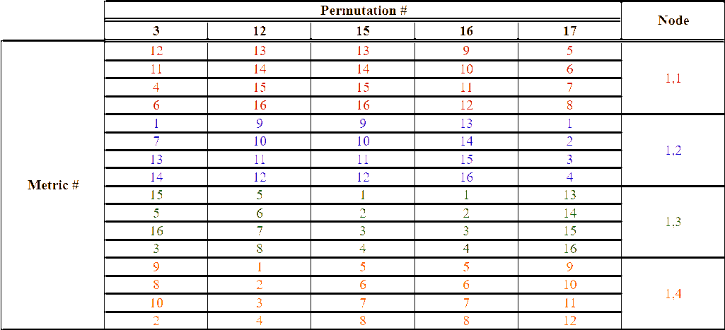
Now we turn to testing the effects of randomly permuting the N = 16 data as it is fed into the network. There were many permutations done to the data and here we discuss the most salient results. All of the permutations to be discussed in this work are shown below in Table 8.

In Table 8, groups of four metrics are highlighted to emphasize which metrics are fed into which bottom-level nodes of the HTM network. For instance, in Permutation #12, metrics 13–16 are fed into the first node in level one (that is, N^1,1). Let us now consider the random permutation to the data (Permutation #3). When we train the same HTM network on this ordering of the data, we get in the top-level node sixty coincidence patterns (C^3,1) and fifty-nine Markov-chains (G^3,1). This is only one fewer pattern than the original network’s top-level node learned. When looking at inference on the training data, we see an identical sequence of Markov-chains indicated by $\text{max}\left[{\lambda }_t\left(g_r\right)\right]$ (see Figure 9).

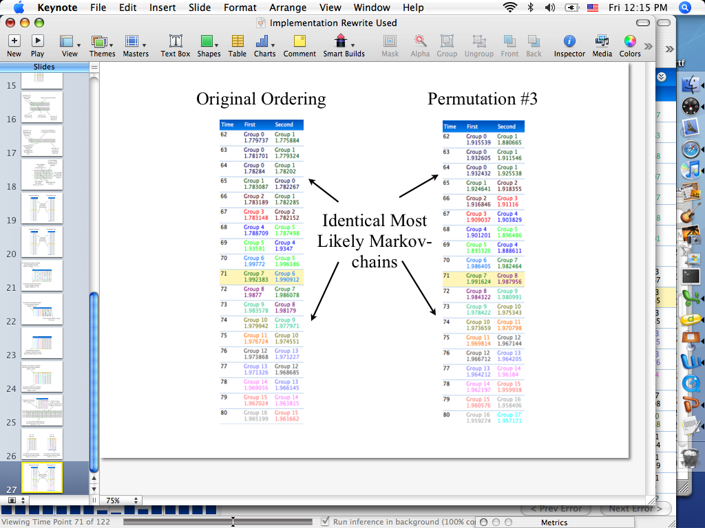
Furthermore, the trend seen in the table continues for all values of t ∈ [62, 122]. As an aside, it is interesting to note that using other system dynamics models for making training data (not shown here), there were changes in this regard [20]. Now, there are none and we see that g0 is recognized as most likely throughout the monotonically stable states. As for the original permutation, during the monotonic unstable states, the progression of most likely Markov-chains is g0, g1, ..., g58. So the network recognizes a progression of increasingly unstable states. But as before, it cannot do so for the increasingly stable ones.

When we look at inference on real data, we see little change in the ability to recognize unstable states. A complete history is shown in another work’s appendix for the top-level node (see appendix C.23 in [20]). For instance, at t ∈ {11,18}, the probability distribution shifts towards higher Markov-chain numbers. This indicates increased instability at these time points, as it has for past observations. For t ∈ {41,43,47}, we see comparable shifts in the probability distribution that we have seen before. But, there are also some time points that we have identified in the past as “unstable” that are not recognized as such right now. For instance, t = 49 has been recognized as such by previous networks, although this network ranks g24 to be only the seventh most likely Markov-chain here. So we see how the results can change slightly based on how the data is permuted when fed into the network. This is likely due to the different hierarchical condensation of data during learning. Overall though, the inference performance on real data bears strong resemblance to what has been seen earlier. Other random permutations of the data can be tested and similar results follow. The progression of recognized unstable states remains monotonic in the top-level node and similar time points are recognized to be closer to instability than others.

In general, it seems that the monotonic training approach is only slightly susceptible to random permutations of the data that violate the hierarchical boundaries imposed by the network. We continue to investigate permutations of the data along those boundaries.

The hierarchical storage of data in the network can be tested with permutations of the data along hierarchical boundaries of the network (for example, Permutations #12, 15–17 in Table 8). First, we use Permutation #16. Here we see top-level coincidence (C^3,1) and Markov-chain (G^3,1) learning that is identical to the original. Also, the inference performance on both data sets is identical at the top-level node. If we compare snapshots of inference on real data side by side then we can see an example of this (Figure 10) for t ∈ [9,27].

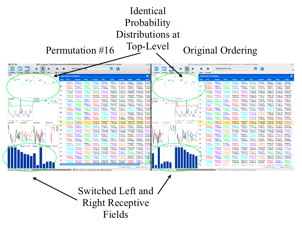
For this permutation, we have only switched the left and right receptive field of the network. Consequently, identical probability distributions in the top-level node indicate that the data is stored hierarchically in the second level of the network. We find the same results when we do this test for Permutations #15, #12 and #17. This result for #15, #12 and #17 indicates hierarchical storage in the bottom-level nodes. Consequently, this means that aspects of instability are hierarchically stored and combined in the network, as it did earlier. Interestingly, for Permutation #13, we see slight changes in the probabilities but the progression of most likely Markov-chains ($\text{max}\left[{\lambda }_t\left(g_r\right)\right]$) is the same as with the original configuration of the data. Recall that Permutation #13 switches the right sub-fields within both left and right receptive fields. Consequently, this permutation violates the hierarchical boundaries between the metrics imposed by the network. So we should expect to see slight changes here, due to the learning mechanisms embedded in HTM nodes. Nevertheless, we see comparable inference performance from the top-level node on the actual data set. A comparison of inference excerpts can be seen below (Figure 11).

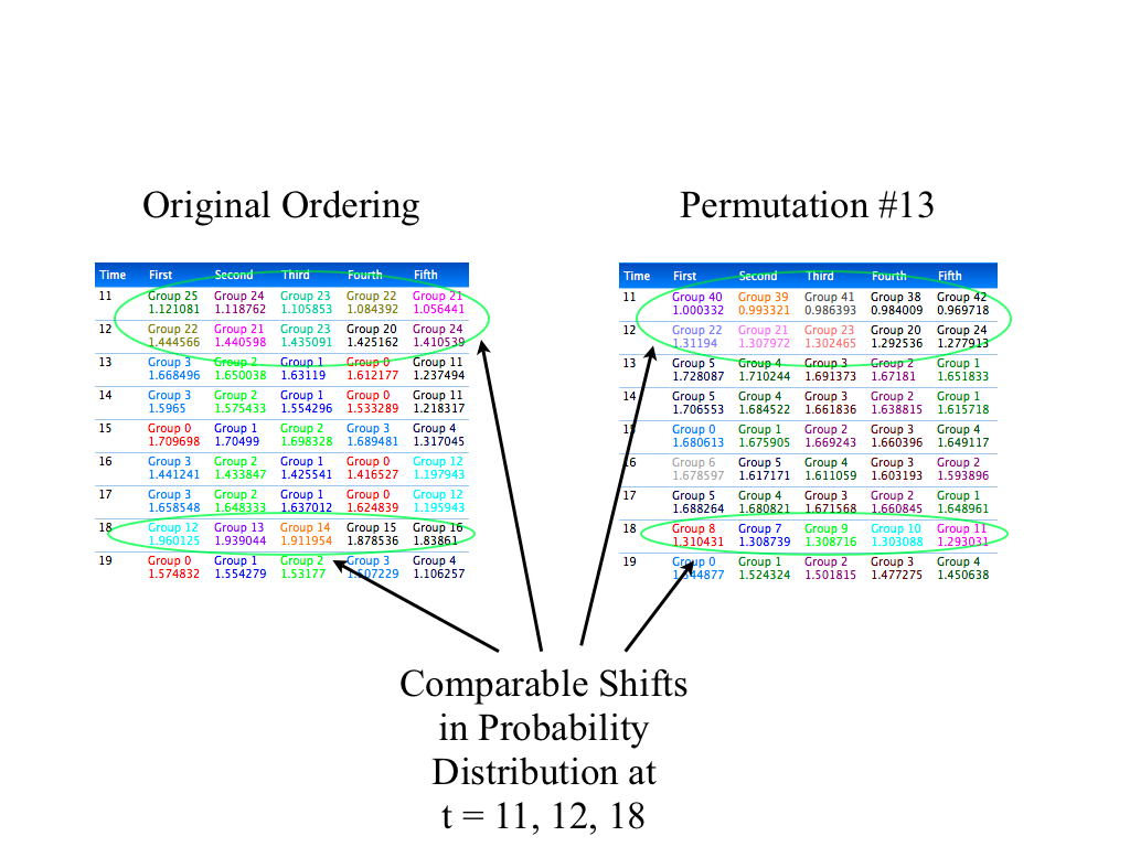
As the figure shows, at t = 11,12,18 there are shifts in the probability distribution towards higher number Markov-chains, indicating heightened instability. This is a familiar result from other networks and other permutations of the metrics, as the figure demonstrates. Furthermore, these comparisons continue for the rest of the inference history.

So we can conclude that, as before, there is little change in the network performance when the data is permuted in groups of four. The only slight change happens for Permutation #13, in which we switch sub-fields within left and right receptive fields. This result was also seen for networks trained on different system dynamics models [20]. Consequently, we can reasonably conclude that there is something about these metrics that makes this happen. Some possible reasons are that the permutation of metrics 5–8 with 13–16 isolates four of the politico-economic metrics within dissimilar other ones. For instance, crude oil production, crude oil export, nationwide electricity and nationwide unemployment are now sandwiched between IED U.S. troop deaths and other hostile-fire U.S. troop deaths. Another possible—and related—reason is that three out of the four politico-economic metrics increase with stability, whereas none of the four metrics they replaced were. This means that during training on monotonic data, these subfields exhibit different end states. We saw before that these end states tend to zero. Consequently, this can also affect learning/inference.

In summary, these tests have revealed details about the training/testing approach done here. We have subjected the network trained on monotonic extreme-cases to these tests and have seen commendable performance. However, there are still many unknowns. Nevertheless, we see intriguing abilities for an HTM network to recognize instability via bottom-up evidence. We should recall that these abilities have been created via training the network on fictitious monotonic data. Then, when we analyse actual data, we are able to categorize the level of instability seen from the evidence. Quantitatively, this categorization is done with the Markov-chain probability distributions in the top-level.

V. comparison to qualitative sa

Using pure data as bottom-up evidence, we have computationally created Level 2 SA in different ways on the Iraq context. We have also seen some consistent results across a broad spectrum of tests and modifications. But how does this compare to what the U.S. Department of Defense (DoD), whose Level 2 SA we are somewhat simulating, wrote about during this time? The reports on Iraq are quarterly and so they evolve over different intervals than the evidence [7]-[18]. Nevertheless, some comparison is possible to judge our networks’ performance in light of these qualitative assessments. For instance, many of the networks examined here have identified fluctuating instability for t ∈ {41,43,47,49}. These time points correspond to October 2006, December 2006, February 2007 and April 2007. Let us examine what the quarterly reports that cover these time periods describe about Iraq.

We begin with a comparison to the November 2006 report [12]. The executive summary of the report provides a good overview comparable to the one we have chosen by looking at N = 16 metrics to describe this complex system. Specifically, the summary focuses on security, political and economic aspects to the stability of Iraq. These are aspects we have considered as well. With regards to security, the DoD writes, “[Progress] is notable given the escalating violence in some of Iraq’s more populous regions and the tragic loss of civilian life at the hands of terrorists and other extremists.” If we look at t = 41, we see that some of this violence is reflected in the evidence (for instance, see appendix C.3 of [20]). Consequently, previous networks indicated this time point as somewhat unstable (for example, see inference output in Figure 6 and Figure 8). With regards to economic stability, the DoD writes, “[The] security situation, maintenance deficiencies, and management issues have adversely affected distribution and delivery of [essential services] ... Electrical distribution was affected by the same problems as the oil sector [.]” The data reflects these problems and many of the HTM networks pick up on this, for instance at t = 41. Of course, the problem is that the mapping between qualitative and quantitative description is never perfect. Nevertheless, these qualitative assessments do not contradict what we have seen thus far from quantitative analysis.

Comparison to the June 2007 report provides some interesting insight [14]. This report covers time points t ∈ [45,48]. Recall that t ∈ [47,49] have been generally identified by networks as somewhat unstable time points, so the overlap in time is not perfect but it will provide some comparison. The DoD writes as follows:

The period covered in this report ... saw a greatly increased effort to secure turbulent areas ... some analysts see a growing fragmentation of Iraq ... Positive indicators include a decrease in civilian murders and sectarian violence ... while negative indicators include the rise of high-profile attacks and expanded use of explosively formed projectiles.

So is this external validation entirely conclusive? No—because there are pieces of evidence indicating stability and other pieces indicating the opposite. But it lends some credibility to the heuristic approach used to establish bounds on the real data. In particular, the arbitrary peg of instability/stability has resulted in both the November 2006 and the June 2007 reports corroborating with the HTM network’s categorizations. Similar trends are seen when comparing network categorization to other reports. So in the absence of any blatant contradiction between network output and report content, we have no grounds for dismissing this approach to computational SA.

Vi. conclusions

In training networks on the Iraq context, we have created a computational SA about it. For this problem, the sixteen chosen metrics do not describe the whole context. Therefore, we have used HTM networks to infer high-level features from a somewhat ill-posed problem. Nevertheless, we used three techniques to test the SA formed about this context. These tests examined reduction in the number of metrics, altering the ordering of the data and examining the hierarchical storage within the network. We found that a minimum number of metrics is needed to form a satisfactory SA. In general, different networks were able to recognize certain degrees of instability from the data when we considered N = 8 metrics or more (that is, N = 16). Also, we showed comparative confirmation of our results from the U.S. Department of Defense (DoD) reports. Although the N metrics do not describe the whole context, it covers many aspects of Iraq’s stability that the DoD considers important. As a result, we see noticeable overlap between the assessments given by the HTM networks and those of the DoD reports. But the analysis is more authoritative when done with extreme-case bounding, and so we lend more credence to that analytic approach for the Iraq context SA. While the results are not perfect, this work has established and investigated a possible new way of analysing states of a complex system. Furthermore, this can be of use for large organizations, such as the U.S. DoD, which make decisions based on complex systems’ data.

References

Authors

Jason Sherwin completed his PhD in May 2010 at the Department of Aerospace Engineering at the Georgia Institute of Technology. Professor Dimitri Mavris was his advisor and mentor since 2005 at the Aerospace Systems Design Laboratory (ASDL). Sherwin has a Bachelor of Arts in Physics from The University of Chicago (2005) and a Masters of Science in Aerospace Engineering from Georgia Institute of Technology (2006). He joined the Department of Biomedical Engineering at Columbia University in Fall 2010 for a research faculty position as Post-Doctoral Research Scientist. E-mail: jason.sherwin@gatech.edu, or jss2212@columbia.edu.

Professor Mavris is the Director of the ASDL and is the Boeing Professor of Advanced Aerospace Systems Analysis in the Department of Aerospace Engineering at the Georgia Institute of Technology. E-mail: dimitri.mavris@ae.gatech.edu. .

References

D. George, “How the Brain Might Work: A Hierarchical and Temporal Model for Learning and Recognition”, Ph.D. Dissertation, Electrical Engineering Department, Stanford University, Stanford, CA, June 2008.
D. George and J. Hawkins, “Towards a Mathematical Theory of Cortical Micro-Circuits”, PLoS Computational Biology, Vol. 5, No. 10, Oct 2009, p. 1–26.
M.R. Endsley, “Toward a Theory of Situation Awareness in Dynamic Systems”, from Ergonomics: Psychological Mechanisms and Models in Ergonomics, ed. N. Moray, Taylor & Francis, USA, 2005.
M.R. Endsley and D.J. Garland, Situational Awareness: Analysis and Measurement, Lawrence Erlbaum Associates, USA, 1996.
M.R. Endsley, “Toward a Theory of Situation Awareness in Dynamic System”, Human Factors, Vol. 37, No. 1, Mar 1995, p. 32–64.
J. Sherwin, “A Computational Approach to Situational Awareness”, Journal of Battlefield Technology, Vol. 13, No. 1, Mar 2010, p. 1–7.
United States Department of Defense, Report to Congress: Measuring Stability and Security in Iraq, July 2005.
United States Department of Defense, Report to Congress: Measuring Stability and Security in Iraq, October 2005.
United States Department of Defense, Report to Congress: Measuring Stability and Security in Iraq, February 2006.
United States Department of Defense, Report to Congress: Measuring Stability and Security in Iraq, May 2006.
United States Department of Defense, Report to Congress: Measuring Stability and Security in Iraq, August 2006.
United States Department of Defense, Report to Congress: Measuring Stability and Security in Iraq, November 2006.
United States Department of Defense, Report to Congress: Measuring Stability and Security in Iraq, March 2007.
United States Department of Defense, Report to Congress: Measuring Stability and Security in Iraq, June 2007.
United States Department of Defense, Report to Congress: Measuring Stability and Security in Iraq, September 2007.
United States Department of Defense, Report to Congress: Measuring Stability and Security in Iraq, December 2007.
United States Department of Defense, Report to Congress: Measuring Stability and Security in Iraq, March 2008.
United States Department of Defense, Report to Congress: Measuring Stability and Security in Iraq, June 2008.
M.E. O’Hanlon and J. H. Campbell, Iraq Index: Tracking Variables of Reconstruction and Security in Post-Saddam Iraq, The Brookings Institution, April 2008.
J. Sherwin, A Computational Approach to Achieve Situational Awareness from Limited Observations of a Complex System, PhD Dissertation, Aerospace Engineering Department, Georgia Institute of Technology, Atlanta, GA, May 2010. [Online Available] http://smartech.gatech.edu/jspui/handle/1853/33955
J.W. Forrester, Road Maps: A Guide to Learning System Dynamics, MIT Open Courseware, USA, 1994.
Anon., Getting Started with NuPIC, Numenta Inc., Menlo Park, CA, Feb 2010.
J.C. Bohorquez et al., “Common ecology quantifies human insurgency”, Nature, Vol. 462, Dec 2009, p. 911-914.
United States House of Representatives, Making Emergency Supplemental Appropriations for the Fiscal Year Ending September 30, 2005, and for Other Purposes, Conference Report 109-72, May 2005.