
Volume 14, Number 1, March 2011
Critical Behaviour In Patterns Of Violence In Afghanistan
- * Defence R&D Canada, Centre for Operational Research and Analysis, 101 Colonel By Drive, Ottawa, ON K1A 0K2, CANADA
Abstract
This paper examines temporal and spatial patterns of violence from a critical systems perspective using data on levels of violent activity in Afghanistan collected daily from 2006 to 2009. Scaling, persistence and intermittency parameters are quantified in the temporal domain. In the spatial domain, the use of a spatial pattern measure ‘symmetropy’ is explored. This study builds upon previous studies suggesting that 1) the conflict exhibits properties of a near critical system when violent incidents are viewed as a point process, and 2) a link exists between spatial structure formation as captured by symmetropy and critical behaviour.
Introduction
The size-frequency distributions of violent events in conflicts appear to follow power law scaling relationships [1–3], which may be an indicator of underlying fractal statistics [4–7]. In particular, it has been demonstrated that insurgent violence in Afghanistan features characteristics of critical behaviour [4] as well as fractal behaviour in the daily time series of coalition casualties [5], consistent with that of self-organized criticality (SOC). Furthermore, there is evidence to suggest that a variety of systems exhibiting such critical behaviour in the temporal domain also display rich pattern or symmetry formation in the spatial domain corresponding to key features of the time series [8,9]. This underscores the requirement to address the possibility of similarly rooted patterns appearing with regard to the locations of violent events [4,5,10,11].
The data set consists of violent incidents, more specifically attacks, recorded daily in Afghanistan from January 2006 to July 2009 by NATO Forces. The incidents comprise a measure of violence consisting of aggregated NATO force reports of engagements, improvised explosive device (IED) attacks and other violent acts. There are 31,475 recorded incidents in the data set overall, averaging 24 per day with a maximum of 82, minimum of 0 and a standard deviation of 13.9. Note, however, that the mean and standard deviation have limited use here given that the data series is non-stationary and is not well described by Gaussian (Normal) statistics [4,5].
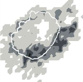
Figure 1 (top) delineates interior (lightly shaded) and exterior locations of violent incidents with respect to the Ring Road in Afghanistan—an important transportation route. The bottom figure shows the density of incidents on a logarithmic (base 10) scale. Both figures clearly demonstrate that violent events are localized along specific portions of the Ring Road, in particular near the border with Pakistan (lower and rightmost sections, Pashtun areas).
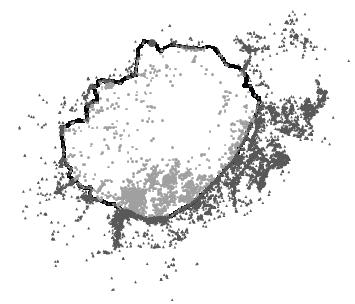
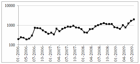
Figure 2 (top) shows the daily counts of violent incidents. The pattern of daily counts appears to have two components. One is the seasonal trend (increase in the incident counts for the summer months), and the other is an overall exponential-like increase in the violent incident counts over time [11]. Average monthly counts are also shown on a log-normal scale (bottom).
We note an important caveat before proceeding further. The data set being analyzed is that of violent incidents (attacks), whereas those previously analyzed for signatures of critical behaviour were of fatalities [4,5]. Although related, they are not the same, and one cannot be assumed to provide a simple proxy for the other. However, given improvements in force protection resulting in reduced fatalities on the side of the coalition, the violent incident counts are a better proxy of the actual combat dynamics than the fatalities. Thus, in light of previous findings for fatalities, the analysis of potentially critical behaviour in violent incidents is important in its own right, as are any ties to the spatial domain.
The analysis of temporal and spatial patterns in the violent activity data provides a much more complete picture of violence in the country that overlays previously computed fatality results. Furthermore, differences in the critical behaviour between the two data sets can be analyzed to theorize on the impact of increasing or decreasing the potential for violent attacks to cause casualties.
The paper is organized as follows. The time series of violent incident data are analyzed for indicators of critical behaviour. The main trends are subtracted before scaling relationships and persistence (long-term memory) within the remaining statistical ‘noise’ are investigated.
Following reference [11], symmetropy is used to examine the spatial signature of the violent events series on a monthly basis. This quantity is computed for both the raw location data and also for the same data transformed to a space where the Ring Road becomes the vertical axis while the horizontal axis coordinate represents a signed distance from the roadway (‘minus’ for events occurring within the interior of the Ring Road and ‘plus’ for exterior events). This strengthens any underlying signal by reducing the pattern signature or ‘footprint’ of the circular roadway itself.
Finally, the spatial and temporal analyses are then compared and contrasted, followed by a discussion and conclusions.
Critical behaviour in the time series of violent incidents
Systems displaying critical behaviour in the time series of events are typified by power-law scaling in the statistical distribution of events (event size – event frequency) and the presence of persistence or long-term memory in the time domain [12]. The former is typically quantified through analysis of the spectral density, wavelets, and/or generalized dimensions, while the latter is often quantified via the Hurst coefficient or some other form of fluctuation analysis.
If the data series under scrutiny is non-stationary, that is, the relevant statistics are not invariant with respect to time translations, then analysis with the measures of choice is problematic [13]. This holds true even with de-trended fluctuation analysis (DFA) [14], which has been demonstrated to show significant bias in general [13], and in particular when challenged with the presence of strong periodicity [15,16]. The seasonal cycles and general exponential-like growth are therefore removed here. Furthermore, the local Whittle estimator [17,18] is used to quantify persistence in place of DFA.
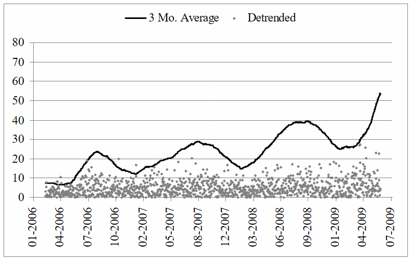
Figure 3 shows the de-trended series of all violent incidences recorded. The trends in the incidence counts were removed by subtracting the three-month (90-day) running average of the counts (the trend line is also shown). The absolute value of the deviation was used in the calculations.
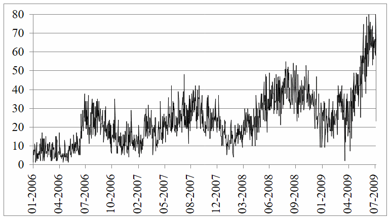
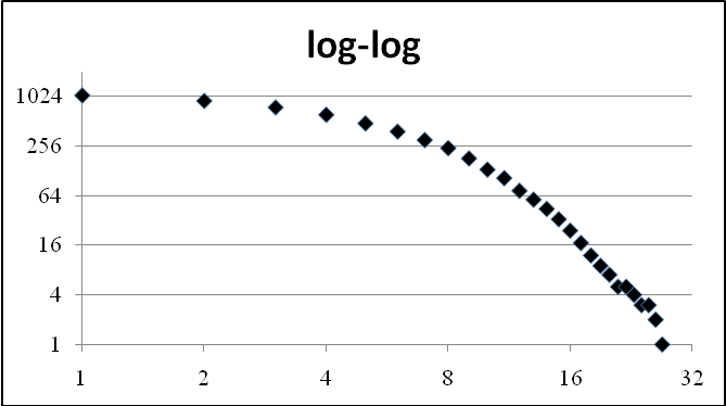
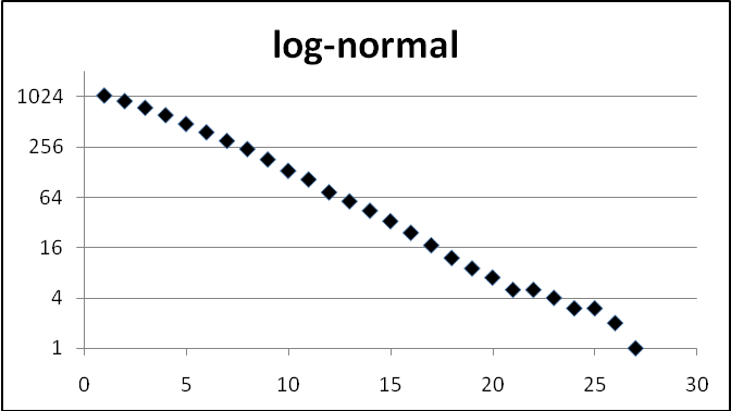
Figure 4 (top) shows a power-law (log-log) plot of the number of occurrences of a given deviation size (or greater) versus deviations in incident count. Fatalities have been identified to be nominally power-law for intermediate event sizes, with deviations from power-law scaling occurring both for large and small events sizes [3]. However, for relatively sparse data sets typical of violent conflict, discriminating against power-law or other heavy-tailed behaviour such as log-normal can prove difficult [2]. The larger data set concomitant to a more inclusive measure of violence appears to be better described by log-normal scaling: the bottom of Figure 4 shows a log-normal plot of the same data, which appears to be an improved fit overall and is a particularly superior descriptor for high frequency incidents (small event sizes). The log-normal transform is quasi-linear, described by y ~ –0.39x + 10.8 (R2~0.995) where y is the number of incidents and x the event size, indicating the log-normal captures the gross characteristics of the violent incidents.
Over the 2006–2009 time period, approximate power law scaling appears only for deviations from the trend with a size greater than ~8 incidents per day, larger than roughly a quarter of the entire data set, and appears jagged beyond 21 incidents per day as a result of finite data effects (Figure 4). The scaling region corresponds also to a lower number of occurrences (frequency). Both log-log and log-normal fits to the data are comparably good in that region, in a naïve sense, yielding R2 values of ~0.99 in both cases.
On the low end, approximate log-normal scaling is most descriptive for deviations from the trend lower than ~8 incidents per day, corresponding to higher frequencies of occurrence (R2~1.0 for log-normal and R2~0.88 for log-log).
Overall, the scaling properties are somewhat consistent with the notion that the data obey a log-normal law over a broad range of sizes and then (possibly) transition to power-law behaviour at very large values of the size variable, as proposed for some systems thought to obey an inverse power law [13,19]. However, the data does not admit enough resolution to directly determine if such a transition actually exists.
The fact that smaller incident sizes do not display power law scaling suggests that there may be some randomness superimposed on the system dynamics, possibly through factors such as environmental conditions, weather, or other random drivers impacting human behaviour.
The high frequency portion of the Fourier power spectrum adds weight to this assertion (Figure 5, top), displaying a ‘flat’ spectrum on average, typical of white-noise. White noise signifies a lack of correlation in the data at those frequencies.
The low frequency region slopes downward on average with a slope of approximately –0.33 (αS ~ 0.33, stderr 0.11), a signature of power law scaling in the parameter αS, although the precise value is widely uncertain in this case.
The flat portion (high frequency) yields a slope of ~ –0.04 (stderr 0.03) making it nearly undistinguishable from white-noise, with zero-slope. This uncorrelated short-time behaviour indicates that random effects are significant, which is consistent with expectations.
The negative slope in the low frequency region suggests ‘1/f noise’, which, incidentally, need not correspond exactly to a power law scaling parameter of α ~ 1, but rather any value in the range 0 < α < 1 is potentially of interest (i.e., 1/f α scaling indicating that there are correlations in the data) [12].
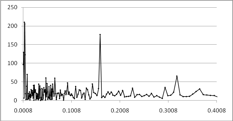
The most significant period that is identified in the periodogram is ~304 days, likely corresponding to seasonal cycles in the external driver. There is also a significant peak near 6.25 days, likely corresponding to a weekly cycle in the external driver (Figure 5, bottom).
A deeper analysis of the scaling properties yields a scaling parameter of αF ~ 0.49 (stderr 0.02), derived from the Fano factor [20] and αA ~ 0.43 (stderr 0.04) from the normalized Haar-wavelet variance (NHWV) [13].
Computation of the second moment of the counting process N(T), where T is the counting window (for example, the total number of incidents within a period of T of one other), provides an estimate of the intermittency C2 and the correlation dimension D2 through the scaling relationship <N2(T)> ~ T2–C2 and the equation relating the two: D2=1–C2 (Figure 6, top) [20]. The value found for D2 is ~0.91 (stderr .01) and for C2 it is ~0.09 (stderr .01). The latter measurement is consistent with [21], also reporting low intermittency in the same data series at ~0.12.
| f | Df | stderr |
|---|---|---|
| –1 | 1.02 | 0.01 |
| 0 | 1.03 | 0.02 |
| 0.5 | 1.03 | 0.02 |
| 1 | 0.98 | 0.03 |
| 2 | 0.89 | 0.01 |
The major implication of the fact that there are two dominant trends—the exponential increase in the numbers of incidents and power law scaling of deviations from this trend—is that there are likely two distinct sets of dynamics at work in the system.
To explore the nature of the dynamics further, the level of persistence (long-term memory) in the system was resolved. A first look at persistence derives from the values already computed, as follows.
By virtue of the fact that D2 does not even approximately equate to αF, the process is not well described as a fractal point process (FPP) [20,13]. Rather, it is more aligned with a fractal rate point process (FRPP), wherein fractal characteristics lie in the rate of counts associated with the point process and the process itself is not fractal. The relationship between FPP and FRPP is one of exclusion. This is consistent with the analysis conducted for the fatalities [5].
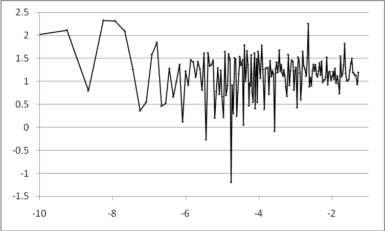
This notion is further bolstered by a plot of the generalized dimension scaling functions [13], which yield values (slopes) for all generalized dimensions near unity suggesting that the process itself is not FPP nor strongly multi-fractal (Figure 6, bottom). Furthermore, the scaling exponent τ(f) = (1–f)∙Df is a linear function of f, indicating a mono-fractal (Figure 7) [22], where the dimensions Df are labelled as follows: {D-1, Dhalf, D0, D1, D′2}. D0 is also known as the capacity dimension and D1 the information dimension. The last member of the set, the correlation dimension, is tagged with an additional ‘prime’ symbol (′) to distinguish it from the value computed for the same quantity (D2) earlier.
The generalized dimensions are determined by the slopes of the rising portions of the various scaling function plots, up until oscillations become overly pronounced. The furthest deviator from unity in the group happens to be D′2, which assumes a value of 0.89 (stderr 0.01). The corresponding scaling function can be seen crossing over the others in Figure 6 (bottom, inset). All other generalized dimensions assumed mean values in the range 0.98 < Df < 1.03 (Table 1).
Since the process is of the fractal rate variety (that is, FRPP), the Fano factor can be used to produce an estimate for the Hurst coefficient, a measure of persistence, through the relation H~(1+αF)/2 [20,13]. Doing so yields H~0.74, indicating a fairly strong degree of persistence. Note that H ranges from 0 to 1 with H<0.5 corresponding to anti-correlated data, H>0.5 indicating correlated data and H=0.5 indicating a lack of correlations (e.g., random walk).
Calculations performed on the de-trended data confirm the previous result, indicating a value of H=0.76 as estimated using the local Whittle method [17], a well established quasi-maximum likelihood estimation technique [18] which is semi-parametric, assuming scaling in the low-frequency limit.
In a separate effort, DFA was computed using the same data set, but without subtracting out the 90-day trend, preferring instead to rely on the consistency of several polynomial orders of DFA analysis to be certain that the results are not a product of the analysis method [10]. The results suggested a high persistence (H~1) and 1/f (pink) noise—a middle ground between uncorrelated data (H ~ 0.5) and the highly correlated Brownian noise (H~1.5). Such exact 1/f noise is often associated with SOC [13]. The authors of the work contend that the high levels of persistence observed in the data translate to some measure of predictability that potentially could be leveraged for projection purposes in a manner reminiscent of weather forecasting (such as ‘hazard forecasting’).
However, as noted periodic trends were not removed and oscillatory components are known to highly affect DFA estimates [16], with pure sinusoids resulting in H=2 (below the period) which mixes with the noise value leading to an apparent Hurst exponent. The seasonal components are significant here (see Figure 2) and may have artificially raised the estimated H value in [10]; our own estimates on the de-trended data indicate H~0.75—better agreement with the value typical for SOC [12]. Nonetheless, both results point to high persistence, whatever the effect of periodicity.
Thus, one can identify two separate dynamics at work. The intensive dynamics appear to be reasonably described by fractal rate process dynamics, consistent with long-term system memory. The extensive dynamics are observable via the seasonal and exponential-like growth and make up a secondary dynamic driven by external factors, a consequence of the fact that the Afghanistan conflict is not a closed system. External factors could range from resources to human behaviour moderators flowing into or out of the system.
In any event, the combination of long-term memory and scaling relationships discovered in the time series of violent events signifies SOC in the temporal domain [12].
To further explore this dual nature of the time series dynamics, we now turn to the spatial domain.
Transforming the incident space
One of the challenges of the data set investigated here is that it contains several characteristic qualities that are driven by geography, communication networks (roads) and other map features rather than by the complexity of the mutual interactions. Thus spatial patterns that arise are constrained by or even embedded within these features.
In the case of Afghanistan, one of the key map features is the Ring Road, and consequently the pattern of incidents reflects a predominantly circular symmetry. To enable a sharper view of the spatial distribution apart from this dominant feature, the incident data were transformed into a more rectangular pattern. First the distance scale was normalized so that the Ring Road corresponded approximately to a unit circle. Then a transformation was applied—a signed distance map that computed the minimum distance of each event from the Ring Road. Negative distances were assigned to locations within the road boundary and positive distances for exterior locations (Figure 8 (top)).
The transformation cuts the (roughly) circular shape near the northernmost point and then unwinds it. The top and bottom of the transformed map correspond to North in real space, with the centre corresponding to the South. The horizontal distribution of the events extends from the centre of the country to a border (on the right). Note that for the signed distance map, the events shown lie within a buffer zone centred on the road (that is, a band of width ~100 km).
Symmetropy of violent incidents
‘Symmetropy’ is used to quantify the degree of structure formation in the spatial distribution of violent incidents. The quantity is a scalar measure of symmetry modelled after Shannon entropy. By decomposing a given two-dimensional intensity map into four types of symmetry (vertical, horizontal, centro (diagonal) and double), symmetropy captures the symmetry of spatially distributed points by virtue of a (complete) two-dimensional discrete Walsh function pattern basis computed on a square grid [8]. The grid divides the space into M × M cells where M = 2q. By treating the resulting spectrum as probabilities, symmetropy is calculated akin to Shannon entropy resulting in a scalar quantification of a pattern.
Symmetropy has been used to analyze spatial patterns relating to SOC arising in sand-pile cellular-automata (CA) [8] and also geologic fault propagation [9].
In the sand-pile CA example, structural formations relate to the locations of cells involved in avalanches. In subcritical states, when viewed through the lens of symmetropy, the locations appear random. However, during the critical steady state, the computed symmetropy values indicate that strong symmetries (formations) are present.
Moreover, critical behaviour in the sand-pile model is typified by power-law scaling relationships and persistence / long-term memory [12]. In particular, the SOC region displays long-term correlations in the frequency domain and high persistence in the time domain. The relevant ‘memory’ of the sand-pile CA resides in the cells, that is, in the distribution of the number of grains of sand in cells. Both deposition events and also the history of avalanches contribute to this ‘memory’. Symmetropy, in a spatial sense, quantifies the ‘degree of relevant memory’ in the system since it is sensitive to the formation of the avalanche patterns.
A key question regarding the violent incidents spatio-temporal series, when viewed through the lens of SOC, is: Where does the memory in the system reside?
Used in the present context, it may be possible to view symmetropy as measuring whether violence events are ‘stacking up’ spatially in such a way as to lend themselves to ‘avalanches of violence’; for example, in campaigns which build up and act as protracted focal points within specific regions. Indeed, this is the central issue addressed in this section.
The incident data from Afghanistan were aggregated by month to enable calculation of the spatial patterns—the daily events were too sparse to yield definitive results. The calculations were conducted for the violent events of Afghanistan as a whole.
The symmetropy results for the violent incidents in the entire country are shown in Figure 9 for both the untransformed (top) and the transformed (bottom) data. The grid resolution in the figures is q=2. Higher values of q displayed similar patterns, although they were less pronounced (as per [23]).
Note that the lower the value of symmetropy, the more pronounced is the symmetry in the pattern. Higher values correspond to (apparent) randomness in the pattern. Symmetropy is herein normalized to yield one as a maximum.
For Afghanistan as a whole, the symmetropy picks up the seasonal fighting cycle, with the winter (off-season) incidents distributed more or less randomly and symmetry breaking—regarded as pattern formation—evident each fighting season (~May–June). This is consistent with the major cycle identified in the periodogram of the time series.
Indeed, higher persistence in the temporal domain seems to roughly correspond with higher structure formation in the spatial domain. And local trends towards randomness in the temporal domain (H → 0.5) seem to be reflected spatially through higher symmetropy values computed over the same periods.
Partitioning the time series data into segments corresponding to low (05/2006-07/2006, 04/2007-06/2007, 04/2008-06/2008) and high (08/2006-03/2007,07/2007-03/2008,07/2008-03/2009) symmetropy, as selected from the transformed map symmetropy plot (Figure 9, bottom) revealed moderate persistence for the time periods corresponding to low symmetropy (Havg ~ 0.62 (std .17)) and a lack of persistence during high symmetropy (Havg ~ 0.53 (std .07)), close to random, uncorrelated behaviour; as estimated by the local Whittle method.
It can be seen that a weak relationship between the spatial structure as measured by symmetropy and the time behaviour (H) exists, on average, however it must be noted that there is fairly high scatter in the estimates, and the values are also sensitive to the particular epochs chosen. The imprecise H estimates can be attributed in part to finite sample effect, with an error expected to scale as 1/sqrt(N), N being the number of samples, which indicates the expected std deviation ratios should be ~1.7 (the number N of data points in the low symmetropy epochs are roughly 91 versus the roughly 263 points in the high symmetropy epochs)—quite close to the value of 2.4 found for the data. Additionally, a low resolution symmetropy calculation was used in selecting the time epochs, which makes it likely that the epochs selected contain a mixture of behaviours near the cut-offs, reducing contrast between “high” and “low” epochs. Thus while some indication of a direct relationship between the time persistence and the spatial symmetropy is evident, the data is not powerful enough to allow us to draw sharper conclusions.
Some interesting insights can be gleaned by examining the individual symmetropy components (Figure 9). Initially, the dominant symmetries in the top figure appear to be varying wildly, suggesting shifting emphasis in diverse parts of the country, likely mostly between east and south. Over the last two and a half years, corresponding to the ‘periodic’ portion of the overall symmetropy, the symmetry components stabilize, with horizontal and vertical symmetries dropping and the centro and double symmetries increasing synchronously. This is consistent with increasing focal points of activity in the south and east during the fighting seasons.
Note that symmetropy does not provide information about the absolute numbers of the incidents, only about the relative densities of incidents spread across a geographical area. Consequently, the results suggest that the internal nature of the insurgency did not change in that sense over the period of 2007–2009. That is, the spatial pattern of behaviour seems to be persistent in its own way (not necessarily in the same sense of the temporal domain as found earlier, however).
Discussion
Analysis of the time series of violent events led to the assertion that scaling relationships are indeed present in the data, in addition to long-term correlations. The high persistence and also the value of the scaling parameter point to SOC behaviour [12].
SOC systems tend to exhibit a build-up of some kind of pressure or stress, later to be released in some form of avalanche event or several avalanches that vary in size, frequency and distribution according to statistical probabilities governed by fractal mechanics. In short, the system is attracted to its critical state.
Consequently, the high persistence of fluctuations about the seasonal trend suggests that increases in violent activity are likely to be followed by much of the same the following day. On the other hand, a decrease in violent activity is likely to persist from one day to the next.
It is curious that the overall violent incident series appears to be better represented by a log-normal relationship rather than a log-log relationship. The log-normal result for violent events is arguably at odds with the results for deaths due to violent events, which are apparently better described by power law scaling overall [3–5]. As mentioned previously, an accurate time series of violent incidents should provide a more refined indictor of the underlying violence dynamics than deaths resulting from such incidents, which measures an escalated level of violence. There is subtle but important difference in what is being measured here versus what is being measured by, for instance, Bohorquez et. al. [3], since the violent events series does not attribute a size to each event (for example, number of resulting deaths)—they are simply counted. In a sense, the former can be attributed to waves of violence in an insurgent environment, and the latter to waves of fatalities from insurgent attacks.
Although well-quantified in the temporal domain, in the spatial domain the idea that the avalanche character of SOC is embedded in the spatio-temporal series of violent events as regular patterns of symmetry and entropy is only partially supported.
Definitely, periods of high violent activity emerge as structural regularities in the spatial domain. However, this would be true also if the system were not an SOC, by virtue of the fact that the events happen around or near geographical features that cannot be filtered out completely. These features define a map pattern, and for the most part symmetropy seems to be reflecting varying densities of the map pattern.
Overcoming trends in pattern formation due to the topography and population density of the area within which the violent events are occurring is a major challenge that must be surpassed if symmetropy is to be used as a reliable spatial indicator of SOC in such a situation, and may not be feasible for the general case. Having that said, there are many other potential applications of symmetropy that do not suffer from such difficulties.
On its own merit, the symmetropy measure is useful as an indicator of the degree of regularity in the spatial structure of events, and can help to identify shifts in both spatial and temporal patterns of events.
At any rate, no formal link is accurately established here between critical behaviour in the temporal series and ‘signatures’ of critical behaviour (for example, regularity in spatial patterns) in the spatial series. However, together they are self-consistent and there is some evidence to suggest that self-organization in the temporal domain may be manifest in structure formation within the spatial domain for the data series studied. Of course, this cannot be said in general for the wide variety of SOC processes found in nature.
Conclusions
The time series of violent events in Afghanistan from 2006 to 2009 strongly displays scaling relationships and long-term memory, which are characteristics of SOC. Furthermore, when viewed as a point process, the series appears to be of the FRPP variety. This could serve as a starting point to further identify specific fractal-based process (FBP) candidates that fit the observed behaviour and would be relevant towards forecasting. However, that task is beyond the scope of this paper. See [13] for more on FBPs.
Symmetropy picked up regularities in the spatial pattern of violent events in direct correspondence with the time-varying density and distribution of events (that is, ‘avalanche activity’).
The signature of symmetropy in a coordinate system transformed from the original for the purpose of unravelling the dominant spatial feature—the Ring Road—increased the sensitivity of the measure as the dominant structure imposed by the Ring Road was reduced.
Some evidence was found to suggest the correspondence of low spatial symmetropy and correlation in incidents in addition to high symmetropy and no correlation in incidents. This finding is suggestive of two general types of violence: violence that is independent (and thus random in space and time) as well as violence that is correlated and localized in space, such as is expected from battle campaigns. Comparing the time (Figure 2) and spatial structure (Figure 8) reveals that the lowest symmetropy (most structured) corresponds to the initial rise in violence starting off the fighting season. A possible explanation relates to well planned initiatives spearheading the fighting season which then break off into more opportunistic and uncorrelated combat later on.
Overall, SOC behaviour was confirmed in the temporal domain, but could not be confirmed or denied in the spatial domain, although some measure of consistency in the relationship between the two domains was demonstrated with regard to activity and temporal vs. spatial regularities.
Future work
Violent incidents from other insurgent conflicts and also conventional conflicts require further investigation, especially in terms of their size-frequency characterization by power law versus log-normal relationships, but also their underlying point process dynamics (for example, type of FRPP).
References
[1] L.F. Richardson, “Variation of the Frequency of Fatal Quarrels with Magnitude”, Journal of the American Statistical Association, Vol. 43, pp. 523–546, 1948.
[2] A. Clauset, C.R. Shalizi, and M.E.J. Newman, “Power–law Distributions in Empirical Data”, SIAM Review., Vol. 51, pp. 661–703, 2009.
[3] J.C. Bohoroquez, S. Gourley, A.R. Dixon, M. Spagat, and N.F. Johnson, “Common Ecology Quantifies Human Insurgency”, Nature, Vol. 462, No. 17, pp. 911–914, 2009.
[4] P. Dobias, “Self-Organized Criticality in Asymmetric Warfare”, Fractals, Vol. 17, No. 1, pp 91–97, 2009.
[5] P. Dobias and K. Sprague, “Intermittency of Casualties in Asymmetric Warfare”, Journal of Battlefield Technology, Vol. 12, No. 1, pp. 19–25, 2009.
[6] M.K. Lauren, “A Fractal-Based Approach to Equations of Attrition”, Military Operational Research, Vol. 7, No. 3, pp. 17–30, 2002.
[7] A. Ilachinski, Artificial War: Multiagent-based Simulation of Combat, World Scientific, 2004.
[8] K. Nanjo, H. Nagahama, and E. Yodogawa, “Symmetropy and Self-organized Criticality”, Forma, Vol. 16, pp. 213–224, 2001.
[9] K. Nanjo, H. Nagahama, and E. Yodogawa, “Symmetropy of Fault Patterns: Quantitative Measurement of Anisotropy and Entropic Heterogeneity”, Mathematical Geology, Vol. 37, No. 3, pp. 277–293, 2005.
[10] J. Wanliss, P. Dobias and K. Sprague, “Detrended Fluctuation Analysis of Combat in Afghanistan”, Journal of Battlefield Technology, Vol. 13, No. 3, pp. 25–29, Nov 2010.
[11] P. Dobias and K. Sprague, “Measuring Complexity and Critical Behaviour in spatial Patterns in Afghanistan”, Journal of Battlefield Technology, Vol. 13, No. 3, pp. 19–24, Nov 2010.
[12] R. Woodard, D.E. Newman, R. Sanchez, B.A. Carreras “Persistent Dynamic Correlations in Self-organized Critical Systems Away From Their Critical Point”, Physica A: Statistical and Theoretical Physics, Vol. 373, No. 1, pp. 215–230, 2007.
[13] S.B. Lowen and M.C. Teich, Fractal-based Point Processes, Wiley, 2005, ISBN-10 0-471-38376-7.
[14] C.K. Peng, S.V. Buldyrev, S. Havlin, M. Simons, H.E. Stanley, and A.L Goldberger, “Mosaic Organization of DNA Nucleotides”, Physical Review E, Vol. 49, pp. 1685–1689, 1994.
[15] C.V. Chianca, A. Ticona, and T.J.P. Penna, “Fourier-detrended Fluctuation Analysis”, Physica A: Statistical Mechanics and its Applications, Vol. 357, Nos. 3–4, pp. 447–454, Nov 2005.
[16] K. Hu, P.C. Ivanov, Z. Chen, P. Carpena, and H.E. Stanley, “Effects of Trends on Detrended Fluctuation Analysis”, Physical Review E, Vol. 64, 2001.
[17] P.M. Robinson, “Gaussian Semiparametric Estimation of Long Range Dependence”, The Annals of Statistics, Vol. 23, pp. 1630–1661, 1995.
[18] K. Shimotsu and P.C.B. Phillips, “Exact Local Whittle Estimation of Fractional Integration”, The Annals of Statistics Vol. 33, pp. 1890–1933, 2005.
[19] E.W. Montroll and M.F Shlesinger, “On 1/f Noise and Other Distributions with Long Tails”, Proceedings of the National Academy of Sciences (USE), Vol. 79, pp. 3380–3383, 1982.
[20] D.R. Bickel, “Estimating the Intermittency of Point Processes with Applications to Human Activity and Viral DNA”, Physica A, Vol. 265, pp. 634–648, 1999.
[21] C.M. Yanofsky and D.R. Bickel, Intermittency of Point Processes in Warfare, Defence R&D Canada, DRDC CORA Contractor Report, 2010 (under review).
[22] H.E. Stanley and P. Meakin, “Multifractal Phenomena in Physics and Chemistry”, Nature, Vol. 335, pp. 405–409, 1988.
[23] K. Sprague and P. Dobias, Behaviour in Simulated Combat: Adaptation and Response to Complex Systems Factors, Defence R&D Canada, DRDC CORA TM 2008-044, Nov 2008.