
Volume 13, Number 3, November 2010
Detrended Fluctuation Analysis Of Combat In Afghanistan
- 1 Department of Physics, Presbyterian College, 503 South Broad Street, Clinton, SC 29325, USA.
- 2 Defence R&D Canada-Centre for Operational Research and Analysis, 101 Colonel By Dr., Ottawa, ON, K1A 0K2, Canada.
Abstract
We have tested the hypothesis that combat related data in Afghanistan for the epoch 2002–2009 demonstrates features of a complex dynamical system. To detect long-term correlations in the presence of trends, we apply detrended fluctuation analysis (DFA), a modern technique for examination of complex systems, to systematically detect and overcome nonstationarities in the data at all time scales. In every instance strong power law correlations were found, and accurate scaling exponents were obtained. It was determined that a measure of predictability was inherent in the dynamics of the system. In other words, there is a history or memory in the signal so that the future dynamics are not random but statistically correlated with past events. We also found an interesting difference in the dynamics of different types of combat events, suggesting the likelihood of different command structure.
Introduction
The complex nature of natural objects has only in relatively modern times been realized. Objects and systems as dissimilar as clouds, mountain ranges, lightning bolts, coastlines, space plasmas, snow flakes, various vegetables, the human lung and brain, and stock markets all display statistical behaviour that can be described by the term ‘fractal.’ The term was coined in 1975 by Benoit Mandelbrot to describe data in natural and mathematical systems which have heavy-tailed distribution functions and a self-similar statistical structure.
There have been a number of previous studies looking at the fractal patterns in casualty data stemming from warfare [1,2,3] and terrorist activities [4]. Recently, several studies were conducted addressing the potential fractal nature of the fatality data from Afghanistan and Iraq. These studies demonstrated that the casualty numbers in these two conflicts obey a power-law distribution; Self-organized criticality (SOC) was suggested as a possible mechanism behind this phenomenon.
Further analysis of the long-term correlations in the fatality numbers from Afghanistan and Iraq confirmed the existence of long-term memory in the systems [5,6]. Since systems with long-term memory obey a power-law, rather than normal, distribution the standard descriptive statistics (such as mean or standard deviation) do not have their usual meaning. The probability of extreme events is much higher than would be expected from a normal distribution. This needs to be taken into consideration for risk assessment and planning.
This paper takes the analysis one step further, addressing the fractal dynamics of various types of significant activities (SIGACTs) in Afghanistan. The data used comprise events occurring in Afghanistan from 2002 to mid 2009.
Our paper is organized as follows. In the first section the general data description is provided, followed by a discussion of the power-law scaling of the daily SIGACT counts in the second section. Then the methodology, with particular emphasis on fractal Brownian motion (fBm) and detrended fluctuation analysis (DFA), is presented. In the fourth section we show the analysis of persistence in the incident counts, and lastly discuss some implications of the results.
SIGACTs data
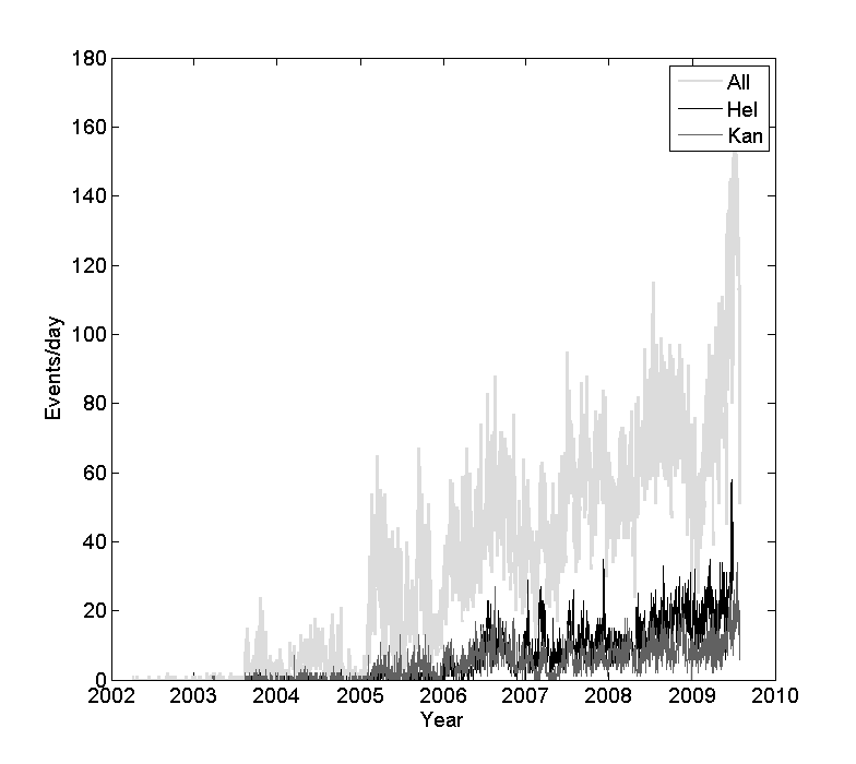
The analyzed data, called the Daily set, comprise the number of selected, combat related events for each day. Because the data record only the number of events for a given day, and not the time of day when the events occurred, it was not possible to create a finer temporal data set. The data for the entire country of Afghanistan, as well as separate data for Kandahar and Helmand provinces, were analyzed. The two provinces were singled out since they were the most volatile areas and were responsible for a significant proportion of the incidents. As the military mission has progressed from the onset of the conflict, the number of enemy contacts and events has increased. Figure l shows the Daily total number of combat incidents in Afghanistan (lightest plot). Total daily events are also recorded for Kandahar (darker) and Helmand (darkest/black).
A significant portion of days recording multiple events is evident from the figure, as is the increasing trend in the daily count of hostilities. These data give evidence of intermittency, and of long-range dependence and nonstationarity. The intermittency is suggested most clearly (because of scale in the figure) by the sudden jumps, or flights in the data for all events (lightest).
This can be seen, for instance, in the sudden jump to over 60 events/day at the start of 2005, or the precipitous decrease at the end of the series from above 150 events/day to below 60 events/day. Long-range dependence is suggested by the longer-period trends, for instance during much of 2009. Aside from the summary data for all SIGACTs, four subsets (violent events, troops in contact (TIC), attempted improvised explosive devices (IEDs) and IED strikes) were analyzed for all three geographical options (all of Afghanistan, Kandahar province and Helmand province).
Power-law scaling of count-frequency relationship of SIGACTs
A number of earlier studies suggested that the fatality counts in Afghanistan obey power-law distribution [4,5]. Figure 2 shows that the incident counts behave in the same manner, however, the scaling coefficient is higher. Furthermore, we observed a different scaling relationship for 2002–06 and 2006–09. This suggests a possible shift in the dynamics around that time.
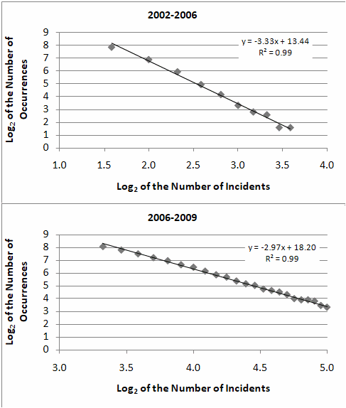
In addition, spectral analysis revealed that the incident counts exhibit 1/f noise characteristic of a near-critical system. These observations suggest the presence of long-term memory in the system.
Detrended fluctuation analysis (DFA)
Long-range correlations can be tested for in numerous ways. A general methodology is to estimate how a fluctuation measure, denoted here by F, scales with the size n of the time window considered. Specific methods, such as Hurst’s rescaled range analysis [7], power spectral analysis, structure function analysis [8], or DFA [9], all essentially calculate such a fluctuation measure, although the measure is different for each technique. For a stationary time series one can apply standard spectral analysis techniques to calculate the power spectrum E(f) of the time series Bα as a function of the frequency f. For long-term correlated data that follows fBm the relationships between the scaling exponents of the various methods are simple. For instance, for stationary data, from spectral analysis we have E(f) ~ f –β where β= 2H – 1 = 1 – γ, with H being the Hurst exponent, related to the correlation exponent γ.
Usually, real-world data are not stationary, and therefore it is generally inappropriate to use techniques like spectral analysis as they are liable to yield unreliable results. For nonstationary data modern methods such as DFA have been developed. Using DFA, the fluctuation function varies in proportion to α (F nα), where α is the scaling exponent. For a time series that tends to follow fBm the relationship is α = H.
For the special case α = 1/2, fBm reduces to the well-known random walk of Brownian motion. Signals with scaling exponents above α=1/2 are also called persistent, because if the data at some point have B(ti+1)>B(ti), for example, then the probability is greater than 0.5 that B(ti+2)>B(ti+1). Signals with exponents below 1/2 are called antipersistent, or anticorrelated, because if B(ti+1)>B(ti), the probability is greater than 0.5 that B(ti+2)<B(ti+1). Typically, fBm is nonstationary, and thus detection of the presence of memory is a delicate task. Nonstationarity means that the statistical properties are not constant through the signal, and traditional analysis methods, that assume stationarity (e.g. power spectra), cannot be used. Notwithstanding the difficulties, fBm has been observed in a variety of fields, including hydrology [11], geophysics [12], biology [13], telecommunication networks [14], and others. We will employ DFA to the combat data to test whether their behaviour is consistent with fBm.
Novel ideas from statistical physics led to the development of DFA [9]. The method is a modified root mean squared analysis of a random walk designed specifically to be able to deal with nonstationarities in nonlinear data, and is among the most robust of statistical techniques designed to detect long-range correlations in time series [15,16,17]. DFA has been shown to be robust to the presence of trends [18] and nonstationary time series [19,20]. This makes DFA appropriate to many natural signals that are heterogeneous, and exhibit different types of nonstationarities. In the case we examine here, the combat data is highly nonstationary displaying all of the complexity inherent in data produced by nonlinear feedback.
Briefly, the DFA methodology begins by removing the mean, , from the time series, B(t), and then integrating:
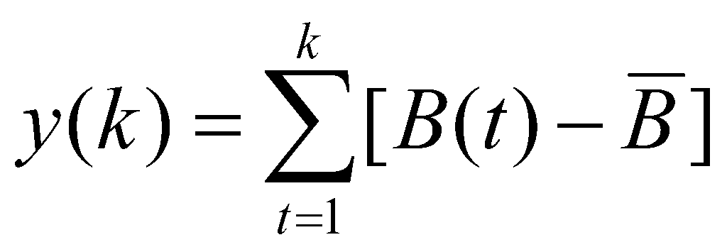
The new time-series is then divided into boxes of equal length, n. The trend, represented by a least-squares fit to the data, is removed from each box. The trend is typically a linear, quadratic, or cubic function [18,21]. Box n has its abscissa denoted by yn,m(k). Next the trend is removed from the integrated time series, y(k), by subtracting the local trend, yn,m(k), in each box. The degree of the trend polynomial can be varied in order to eliminate constant (m=0), linear (m=1), quadratic (m=2) or higher order trends of the polynomial function. Conventionally, the DFA is named after the order of the trend function polynomial (DFA0, DFA1, DFA2, ...). In DFAm, trends of order m in the polynomial fitting function and of order m–1 in the original record are removed.
For a given box size n, the characteristic size of the fluctuations, denoted by F(n), is then calculated as the root mean squared deviation between y(k) and its trend in each box
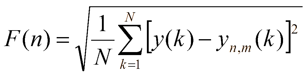
This calculation is performed over all time scales (box sizes). A power-law scaling between F(n) and n indicates the presence of fractal scaling:
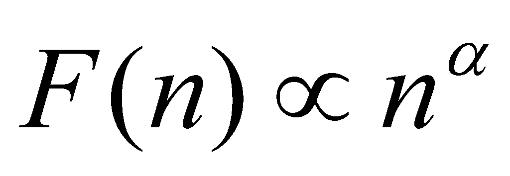
where the parameter α is a scaling exponent. The scaling exponent can take values between 0 and 3/2; if α=0.5 the signal is white noise and there is no correlation in the data; α<0.5 indicates anti-correlation, meaning that large values are most likely to be followed by small values and vice versa. Values of α>0.5 indicate a correlated time series. The larger the value, the more persistent and smooth is the time series. Visually, anti-correlated data presents a rough profile in comparison to smoother profiles with correlated data. When α=1 the signal corresponds to ‘pink noise’. Pink noise relates to a time series with a 1/f power spectrum, although as we mentioned above the nonstationary nature of the data would render spectral analysis spurious. Numerous mechanisms and processes produce 1/f noise in nature and in human physiology [22]. When α>1, correlations still exist in the system, but they are not of a power law form and α=1.5 corresponds to ‘brown noise’—the integration of white noise.
Persistence in the SIGACTs
In any numerical analysis of real data one must always be conscious of the caveats intrinsic to a given methodology. This assumes, naturally, that the methodology may be legitimately applied. For instance, for nonstationary data spectral methods are inappropriate and will yield results that are spurious or without merit. On the other hand, for our data the methods introduced in the previous section yield results that are trustworthy, provided care is taken to test for all possible causes that can make the method fail. In short, to understand the intrinsic dynamics of a given system, it is important to analyze and correctly interpret its output signals. Many records do not show simple monofractal scaling, but in other cases there are crossover timescales separating regimes with different scaling exponents. For example, there can be one type of correlation at long timescales and another at small scales. To be sure one can reliably detect long-range correlations, it is important to differentiate trends from the long-range fluctuations intrinsic in the data. An artificial crossover in the fluctuation function usually can arise from a change in the correlation properties of the signal at different time or space scales, or can often arise from trends in the data. Trends can thus lead to a false detection of long-range correlations. In thinking of the combat arena in terms of a complex physical system, one needs to recognize that trends may arise from the intrinsic dynamics of combat rather than being an epiphenomenon of external conditions. As more of the enemy become involved in the combat effort, one might initially expect an increasing trend for conflict that might be smooth and monotonous or slowly oscillating.
Recall the trend over time evident in Figure 1 for an increase in the number of recorded events each day. There is a corresponding downward trend in the time between events. Application of the DFA2 method to noisy signals without any polynomial trends leads to scaling results identical to the scaling obtained from the DFA1 method, with the exception of some vertical shift to lower values for the root mean squared fluctuation function. Similarly, polynomial trends of order lower than l superposed on correlated noise will have no effect on the scaling properties of the noise when DFAl is applied. Because of the obvious presence of trends in the data we therefore applied DFA1, DFA2, and DFA3 to be certain that our results are not a product of the analysis method. It is essential in the DFA-analysis that the results of several orders of DFA are compared as results are only reliable when above a certain order of DFA they yield the same type of behaviour.
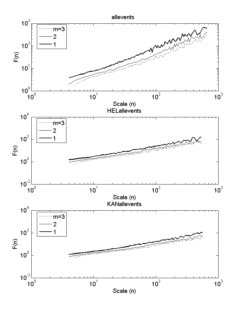
Figure 3 shows the fluctuation function computed for all SIGACTs since 2002. The top graph shows the fluctuation curves for the entire Afghanistan, the middle graph shows curves for all Helmand, and the bottom graph for Kandahar. The top, middle, and bottom curves correspond, respectively, to m=1, 2, 3 for DFAm. Small deviations from the scaling law (Equation 5), i.e. deviations from a straight line in a double logarithmic plot, occur for small scales n, in particular for DFAm with large detrending order m. These deviations are intrinsic to the usual DFA method, since the scaling behaviour is only approached asymptotically. The deviations limit the capability of DFA to determine the correct correlation behaviour in very short records and in the regime of small n.
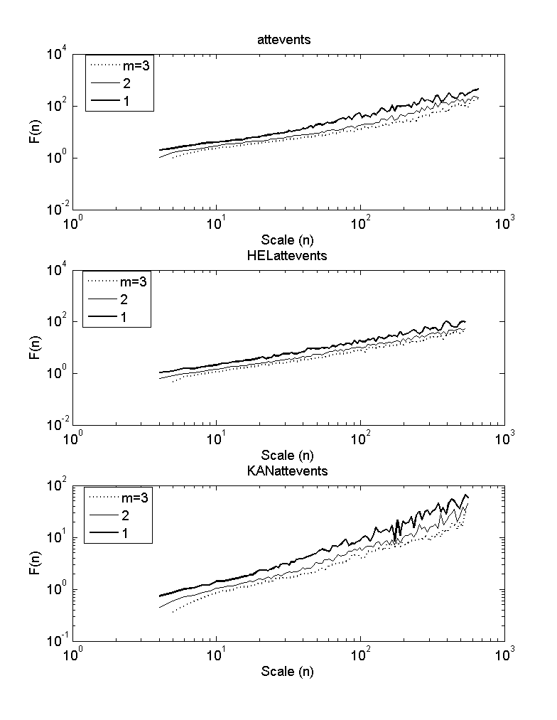
For interest, Figure 4 shows the curves for violent events. Since curves for the other events display essentially the same type of power law behaviour, they are not shown. Table 1 gives the results for the scaling exponents derived from these various curves.
| Data type | α | R |
|---|---|---|
| All SIGACTS | 1.093±0.016 | 0.9922 |
| Helmand All | 0.986±0.017 | 0.9893 |
| Kandahar All | 0.995±0.012 | 0.9947 |
| Violent Events All | 1.200±0.017 | 0.9923 |
| Violent Events Helmand | 0.982±0.016 | 0.9900 |
| Violent Events Kandahar | 0.9840±0.020 | 0.9852 |
| TIC Helmand | 0.973±0.016 | 0.9900 |
| TIC Kandahar | 0.988±0.019 | 0.9859 |
| IED Attempt Helmand | 0.588±0.014 | 0.9819 |
| IED Attempt Kandahar | 0.620±0.011 | 0.9876 |
| IED Strike Helmand | 0.603±0.021 | 0.9580 |
| IED Strike Kandahar | 0.676±0.011 | 0.9912 |
All SIGACTs (the first three rows of Table 1) have a scaling exponent α≈1, within the error. This is a remarkable result that suggests these data correspond to 1/f noise (which is consistent with the results of the spectral analysis, as discussed above), the implications of which will be discussed in the conclusion. All violent events and TICs between Helmand and Kandahar are statistically similar. Indeed, with the exception of IED-related events, there are no statistical differences between the different subsets of events in Helmand and Kandahar. There is a small, but significant, difference in the IED-related events between Helmand and Kandahar.Both Helmand and Kandahar IED combat events also deviate drastically from the rest of the data, having scaling exponents α~0.6. This indicates the presence of a different kind of dynamics governing these events.
Conclusions
In this paper, the nonstationary SIGACT data from Afghanistan were found to exhibit power-law scaling consistent with the presence of long-term memory in the time series. To determine the nature of this long-term memory, DFA was applied to the analyzed data. The DFA served to avoid spurious detection of correlations resulting from data nonstationarity. The idea of the method is to subtract possible deterministic trends from the original time series and then analyze the fluctuations of the detrended data.
In all cases we found that the detrended fluctuation functions were linear over about two decades in log-log space, and no crossover in scaling behaviour was observed. The results indicate that a universal long-range power-law correlation may exist which governs Afghanistan combat variability at all temporal scales. In every instance, strong power law correlations were found in the data, and the appropriate scaling exponents, α, were extracted. In all cases, the scaling coefficient α was greater than 0.5, indicating long-range correlations. This suggests that the size of combat events is correlated; a large offensive is slightly more likely to be followed by increased hostilities the following day, than a decrease in hostilities. On the other hand, a decrease in hostilities is likely to persist from one day to the next. In addition, with the exception of the IED-related events having a scaling coefficient α~0.6, the scaling coefficients were around one (1) suggesting the presence of 1/f noise (which was indeed observed). A significantly lower scaling coefficient for the IED-related incidents suggests that a different dynamics may be at work for these events, perhaps suggesting a different command structure. This result, which points to the likelihood of different dynamics in different regions, is probably the result most immediately useful. In summary, the findings strongly suggest that the SIGACTs in Afghanistan exhibit the properties of SOC and that in terms of the SIGACTs, the conflict is in a critical state.
The important message to take from this analysis is that there is a measure of predictability inherent in the dynamics of the combat system—there is a history or memory in the signal so that the future dynamics are not random, but rather they are statistically correlated with past events in a consistent manner. This is seen most strongly for the violent events and TICs, and only weakly for the IED-related events. Consequently, the correlations found may be amenable to modelling after the manner outlined in [23] and [24], although more data may be needed to achieve adequate statistical plausibility to the hazard forecasts. Thus, just as in weather forecasts, one might produce combat forecasts with probabilities assigned to certain events that may provide value-added information for risk assessment.
References
[1] D.C. Roberts and D.L. Turcotte, “Fractality and Self-Organised Criticality of Wars”, Fractals, Vol. 6, 1998, pp. 351–357.
[2] L.F. Richardson, “Frequency of Occurrence of Wars and Other Fatal Quarrels”, Nature, 148, 1941, pp. 598.
[3] M.K. Lauren, On the Temporal Distribution of Fatalities and Determination of Medical Logistical Requirements, Defence Technology Agency (DTA) Report 187, NR 1377, ISSN 1175-6594, 2003.
[4] J.C. Bohorquez, S. Gourley, A.R. Dixon, M. Spagat, and N.F. Johnson, “Common Ecology Quantifies Human Insurgency”, Nature, Vol. 462, 2009, pp. 911–914 , doi 10.1038/nature08631
[5] P. Dobias, “Self-Organized Criticality in Asymmetric Warfare”, Fractals, Vol. 17, No. 1, 2009, pp. 91–97.
[6] P. Dobias and K. Sprague, “Intermittency of Casualties in Asymmetric Warfare”, Journal of Battlefield Technology, Vol. 12, No. 1, 2009, pp. 19–25.
[7] H.E. Hurst, “The long term storage capacity of reservoirs”, Transmissions of American Society of Civil Engineers, Vol. 116, 1951, pp. 770–808.
[8] V.I. Abramenko, V. B. Yurchyshyn, H. Wang, T. J. Spirock and P. R. Goode, “Scaling Behaviour of Structure Functions of the Longitudinal Magnetic Field in Active Region on the Sun”, Astrophysical Journal, Vol. 577, No. 1, 2002, pp. 487–495.
[9] C.-K. Peng, S. Havlin, H. E. Stanley, and A. L. Goldberger, “Quantification of Scaling Exponents and Crossover Phenomena in Nonstationary Heartbeat Timeseries”, Chaos, Vol 5, No. 1, 1995, pp. 82–87.
[10] B.B. Mandelbrot and J.W. Van Ness, “Fractional Brownian Motions”, Fractional Noises and Applications, SIAM, Vol. 104, 1968, pp 422-437.
[11] S.P. Neuman and V. Di Federico, “Multifaceted Nature of Hydrogeologic Scaling and its Interpretation”, Reviews of Geophysics, Vol 41, No 3, 2003, pp. 1014–1045, doi:10.1029/2003RG000130.
[12] U. Frisch, Turbulence, Cambridge University Press, New York, 1997.
[13] J.J. Collins, C.J. De Luca, “Upright, Correlated Random Walks: A Statistical-biomechanics approach To Human Postural Control System”, Chaos, Vol. 5, No. 1, 1994, pp. 57–63.
[14] M. Taqqu, V. Teverovsky, and W. Willinger, “Is Network Traffic Selfsimilar or Multifractal?”, Fractals, Vol. 5, 1997, pp. 63–73.
[15] M.S. Taqqu, V. Teverovsky, and W. Willinger, “Estimators For Long Range Dependence: An Empirical Study”, Fractals, Vol. 3, 1996, pp. 785–798.
[16] M.J. Cannon, D.B. Percival, and D.C. Caccia, et al., “Evaluating the Scaled Windowed Variance Methods for Estimating the Hurst Coefficient of Time Series”, Physica A, Vol. 241, No. 3-4, 1997, pp. 606–626.
[17] H. J. Blok, “On the nature of the stock market: Simulations and experiments”, Ph.D. thesis, University of British Columbia, Vancouver, British Columbia, Canada, 2000.
[18] K.Hu, P. C. Ivanov, Z. Chen, P. Carpena, and H. E. Stanley, “Effect of Trends on Detrended Fluctuation Analysis”, Physical Review E, Vol. 64, 2001, doi:10.1103/PhysRevE.64.011114.
[19] J.W. Kantelhardt, S.A. Zschiegner, E. Koscielny-Bunde, S. Havlin, A. Bunde, and H.E. Stanley, “Multifractal Detrended Fluctuation Analysis of Nonstationary Time Series”, Physica A, Vol. 316, No.1-4,2002, pp. 87–114.
[20] Z Chen, P.C. Ivanov, K. Hu, and H.E. Stanley, “Effect of Nonstationarities on Detrended Fluctuation Analysis”, Physics Reviews E, Vol. 65, 2002, doi:10.1103/PhysRevE.65.041107. http://docs.google.com/viewer?a=v&q=cache:y1wQLpuGPhUJ:polymer.bu.edu/hes/articles/cihs02.pdf+Effect+of+nonstationarities+on+detrended+fluctuation+analysis&hl=en&gl=us&pid=bl&srcid=ADGEESgc7rO_LGK848p2cXTNjPa7HXfzbsbfPcbzF2jwZL1YIj7L4HTw0tb_dnqfBusUHvOjB2GDCGAcIofFavxYmSetgFsGzdsegDt2svsFiumAXxYGTFxTt_eMaeLjTTI8wdKe9HQb&sig=AHIEtbSci1i5jBITDdf2EKfix5Tbq0ibWg
[21] D. Vjushin, R.B. Govindan, R.A. Monetti, S. Havlin, and A. Bunde, “Scaling Analysis of Trends Using DFA”, Physica A, Vol. 302, No. 1–4, 2001, pp. 234–243.
[22] B.J. West, V. Bhargava, and A.L. Goldberger, “Beyond the Principle of Similitude: Renormalization in the Bronchial Tree”, Journal of Applied Physiology, Vol. 60, No. 3, 1986, pp. 1089–1097.
[23] J.A. Wanliss, “Multifractal Modeling of Magnetic Storms Via Symbolic Dynamics Analysis”, Journal of Geophysical Research, Vol. 110, 2005, doi:10.1029/2004JA010996, http://www.agu.org/journals/ABS/2005/2004JA010996.shtml.
[24] V. Anh, Z.-G. Yu, and J.A. Wanliss, “Analysis of Global Geomagnetic Variability”, Nonlinear Processes in Geophysics”, Vol. 14, 2007, pp. 701–708.
[25] A. Clauset, C.R. Shalizi, and M.E.J. Newman, "Power-law distributions in empirical data" SIAM Review 51(4), 661-703 (2009). (arXiv:0706.1062).
[26] Koscielny-Bunde, Eva, A. Bunde, S. Havlin, H. E. Roman, Y. Goldreich, and H.-J. Schellnhuber, “Indication of a Universal Persistence Law Governing Atmospheric Variability,” Phys. Rev. Lett., 81, pp. 729–732, 1998.