
Volume 13, Number 2, July 2010
Dynamic Estimation Of Effective Chaff Dipoles In Chaff-Missile Naval Engagement Simulation
- 1 Both authors are with Institute for Systems Studies and Analyses, Metcalfe House, Delhi-110054, India.
Abstract
In a chaff missile engagement scenario the number of chaff elements or dipoles in the missile seeker radar resolution cell (RRC) changes dynamically. To capture this effect in simulation a technique is proposed in this paper to estimate the number of effective chaff dipoles. Estimation using this technique caters for the dynamically changing positions and dimensions of both the chaff cloud and the missile seeker RRC. This proposed technique is based upon the Monte-Carlo simulation method, and its validation has been completed by comparing the analytically computed and the estimated values for different geometric positions of the systems. A chaff missile engagement scenario has been simulated to show the application potential of this technique in estimating the chaff cloud radar cross section (RCS).
Introduction
In modern warfare scenarios, sea skimming missiles are the most critical challenge to the naval force. Defence against such weapons is difficult and expensive. Among all the defensive measures, chaff is probably the oldest (in use since 1937) [1], quite inexpensive, and yet still effective. Generally, chaff can be made of aluminium strips, zinc coated fibre glass, copper wire, and aluminium coated fibreglass. Chaff can either act as a decoy target, or can saturate an area to confuse the radar system [2]. Even for search radar with a relatively long scan period (with or without an MTI processor), valuable time is wasted due to chaff as it takes at least two scans to develop a velocity estimate [3].
Chaff is effective if it provides maximum radar cross section (RCS) in the missile seeker in the shortest possible time. This depends on the timing of chaff launch, the quantity to be dispensed, the initial launch force, and many other parameters. Hence, to use chaff effectively in different engagement scenarios all the crucial parameters have to be identified through analysis. Conducting field trials is not suitable as it is very high in cost, time, environmental hazards, risk, and furthermore, sometimes the scenario to be analyzed itself is not feasible. Simulation is a proper tool for such analysis as it is not only efficient, economic, and safe, but it also gives the freedom to experiment with scenarios which had not been previously thought of. However, capturing the realistic behaviour of the chaff cloud in simulation is complicated due to the dynamically changing scenario and diverse properties of the resonating elements (dipoles).
Most of the earlier works in chaff are related to the study and estimation of different properties of the chaff dipoles. Estimation of their concentration, mutual coupling, wave attenuation, fibre density, polarization, dynamic distribution, and configuration have been done in [4−11]. The basic working principle, common types of chaff and their application has been explained in [12−15]. A technique to simulate the chaff cloud taking into consideration the dispersion, scattering and estimating these by using spatial Gaussian distribution has been proposed in [16]. For the estimation of chaff cloud RCS, simple techniques are explained in [13,17] and fuzzy logic based estimation has been given in [2].
In the chaff cloud RCS estimation methods the number of chaff dipoles is an important parameter. In realistic scenarios the number of chaff dipoles in the missile seeker radar resolution cell (RRC) has been observed to change dynamically. In order to capture this effect in simulation a technique to estimate the number of effective dipoles is proposed in this paper. However, this technique does not restrict the approach to estimate the chaff cloud RCS; it can be used in any model where the effective number of chaff dipoles is needed. To show the application of the proposed technique, a scenario consisting of a point mass missile model tracking a fictitious point in the chaff cloud (chaff centroid) has been simulated. In the simulation run, the estimated effective number of chaff dipoles and the chaff cloud RCS considering the scattering, bird nesting, and polarization properties of the dipoles have been observed.
The rest of the paper has been organized as follows: the classical technique to estimate the number of effective chaff dipoles using a generic chaff RCS estimation model and the need to develop a new technique is explained in Section II. The mathematical interpretation of the problem, difficulties in tackling the problem analytically and the proposed technique is presented in Section III. The validation of the proposed technique is presented in Section IV by comparing the estimated and analytically computed values. The application potential of the proposed techniques and results are given in Section V.
Classical method to estimate the effective number of chaff dipoles
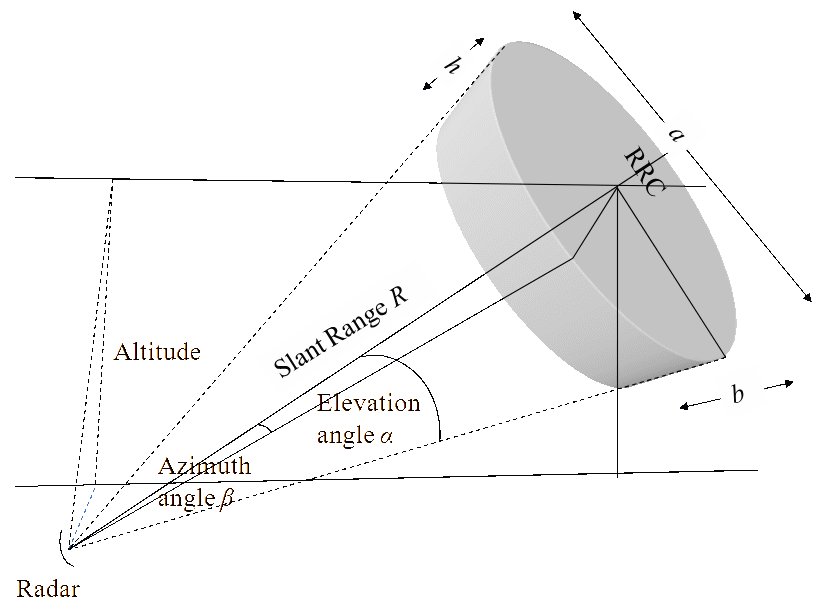
Before describing the classical estimation method, missile seeker RRC and a generic method of estimating the chaff RCS has been explained. RRC is an indication of the radars ability to resolve multiple targets. Its height (h), the azimuth resolution (a) and the vertical resolution (b) are the functions of radar pulse width (Pw), range (R) to the point in the space where the cell is centred, the horizontal beam width (α), and the vertical beam width (β) (see Figure 1). It is clear from Figure 1 that, the RRC spatial volume is delimited by the pulse length and beam shape can be represented by a section of an elliptic cone.
For estimation of the chaff cloud RCS, a chaff cloud with N number of dipoles in the payload has been considered. The RCS of a single chaff dipole σd at first resonance depends on the frequency (or wavelength) and different orientations of the dipoles [12]. Logically, it appears that the RCS of the chaff cloud is equal to the sum of the RCS of the individual dipoles; however the effective RCS observed will be less than this value. Three effects contribute to the deviations from this simplistic response model [18]:
- Dispensing and packaging techniques result in two or more dipoles clinging together to give a response less than the sum of individual responses. This phenomenon is called bird nesting.
- Dipoles within two wavelengths of each other do not behave like isolated dipoles because the field of a single dipole is changed by coupling effects with neighbouring dipoles.
- Dipoles on the near side of the cloud shield the dipoles on the far side of the cloud from the full incident energy of the radar beam. Furthermore, the vertical attitude dipoles fall faster and the chaff cloud RCS depends on the radar signal polarization.
To cater for these effects three factors nf, ne, and npol, are defined; these are the effectiveness factors relating to the behaviour of chaff cloud [2]. The parameter ne quantifies the effect of different launch techniques; for pyrotechnically launched chaff ne≈0.8, while for mechanically launched ne≈1.0. The parameter npol takes into account the effect of single polarization; for horizontal polarization npol≈0.6, for vertical polarization npol≈0.4 and for circularly polarized waves npol≈0.5. The parameter nf models the effectiveness of the dispersion technique and 0.4< npol <0.5.
Using these three parameters the RCS σ of the chaff cloud can be estimated by some functional form φ:

where, A is the area of the radar beam associated with the RRC of interest and n represents the number of effective chaff dipoles. The effective chaff dipoles are those that are within the missile seeker RRC. Only these elements affect the observed RCS of the chaff cloud. In realistic scenarios, the number of effective dipoles changes dynamically as the size and position of both the chaff cloud and missile seeker RRC varies at each instant. Variation in the RRC is observed because of the high velocity and manoeuvrings of the missile in tracking the chaff centroid. The dimension of the chaff cloud changes until the blooming time, then it maintains its shape and size. However, its position changes due to the direction of wind and steady sinking due to gravity. Taking the total number of dipoles in the payload to be effective is correct only when the chaff is wholly within the RRC of the missile seeker. This is usually true at the long ranges, but at short ranges the RRC becomes smaller and only a portion of the chaff cloud will be within it. The classical method of estimation of number of effective chaff dipoles when chaff cloud is larger than RRC is [2]:
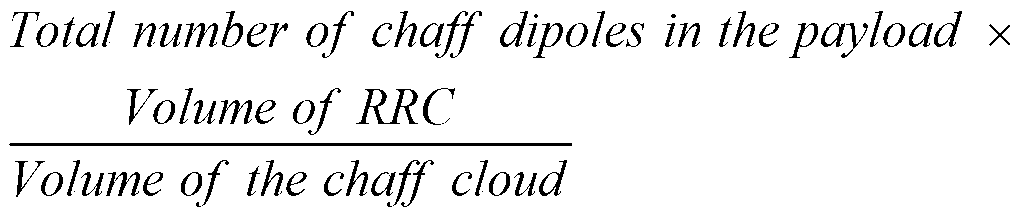
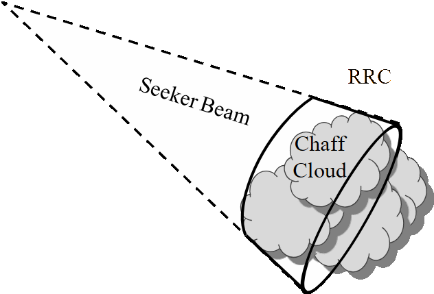
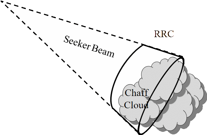
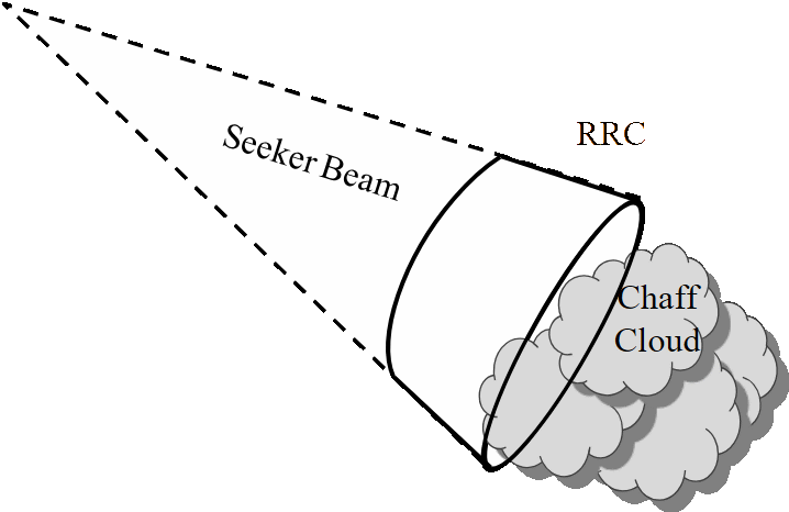
To observe the estimation using this technique three cases; case-A, case-B and case-C (shown in Figure 2(a), 2(b) and 2(c)) are considered. In each of the cases, the volume of the chaff cloud and the RRC are kept unchanged but the position of the chaff cloud is slightly different. In case-A, as the major portion of the chaff cloud is within the RRC, the maximum number of dipoles is effective. In case-B, a relatively smaller portion of the cloud is within the RRC, so a smaller number of dipoles is effective. In case-C, only a small portion of the cloud is within the RRC, so the least number of dipoles is effective.
However, using the classical estimation, the number of effective dipoles is equal in all of the cases, as the volume of both the chaff cloud and the RRC are unchanged, and the number of dipoles in the payload is fixed. Hence, the classical estimation technique is not able to capture the effect of different orientations of the systems. Therefore, there is a need to develop an estimation technique to cater for such cases. In this paper, a new technique has been proposed to estimate the number of effective dipoles for dynamically changing positions and sizes of the RRC and the chaff cloud.
Proposed technique to estimate the effective number of chaff dipoles
As mentioned in Section II, the classical technique for effective dipoles estimation is not able to capture the effect of dynamically changing positions of the chaff cloud and the missile RRC. The technique proposed in this paper caters for both the changes in dimension and position of the systems. The proposed technique estimates the number of effective chaff dipoles at any instant as the product of the fraction of the chaff cloud volume intercepted in the missile seeker RRC at that instant and the number of dipoles in the payload—that is:

The main problem lies in finding the fraction of the volume of chaff cloud intercepted in the missile seeker RRC. A technique for determining this volume has been proposed in this paper. The mathematical interpretation of the problem and the stepwise explanation of the proposed technique is illustrated in the following subsections.
Assumptions and mathematical interpretation
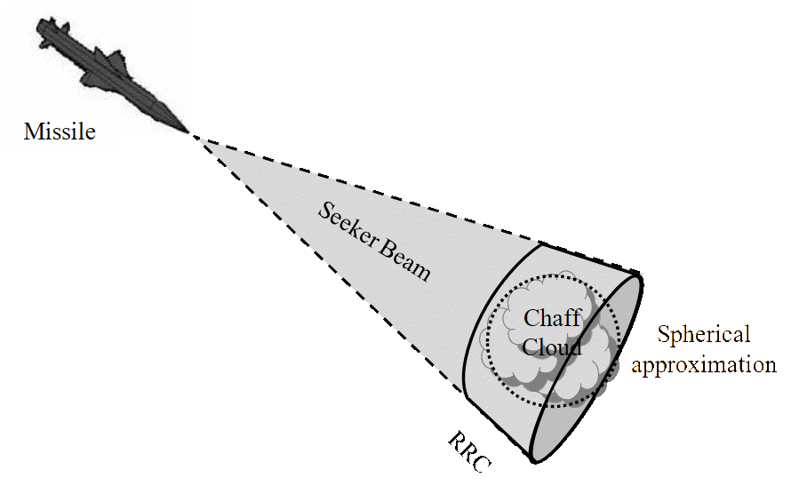
Defining the shape and size of the chaff cloud is very complicated as it depends on many factors like the type of ejection system, the strength given to the ejection, payload weight, varying air densities, wind direction and speed and on the altitude where the chaff is deployed. In the naval scenario the chaff cloud is usually deployed so close to the sea surface that the difference between air densities from where the cloud blooms to the sea surface is negligible. Furthermore, a pyrotechnical ejection system produces a spherical cloud [2]. Hence, in the naval scenario the chaff cloud can be geometrically represented by a sphere. As already discussed in Section II, the RRC spatial volume can be represented by a section of the elliptic cone.
Under these assumptions, the problem is transformed to mathematical/geometrical domain as finding out the fraction of the sphere volume intercepted in the section of elliptic cone. The spherical approximation of chaff cloud is shown in Figure 3. Analytical approach to compute the whole intercepted volume is [19]:
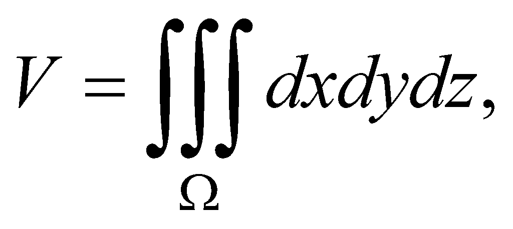
the limit Ω of the variables should embrace the whole solid.
In the missile–chaff engagement scenario, the positions and the dimensions of both the section of cone and sphere is dynamically changing, there are vast possibilities in how interception between them would take place. Due to this the bounding surface and the values of the parameters will be different at each instant. Depending on the bounding surface the projection planes will also be different. Therefore, triple integration having different functional representations and parameters as variable limits is needed at each instant to compute the dynamically changing intercepted volume. Hence, an analytical approach is not suitable for this purpose. Therefore, a simulation technique using a Monte-Carlo method has been used to solve this problem.
Estimation of intercepted volume using Monte-Carlo method
In this paper, the following convention for measurement of angles has been adopted. The angles in the azimuth plane are measured from x-axis to anticlockwise, and the angles in the elevation plane are measured from azimuth plane to positive z-axis.
The cone and the sphere can be oriented anywhere depending on the azimuth, elevation and the range factors with reference to the ground fixed reference system. The scenario is first reduced to the standard form and then the Monte-Carlo method is applied. Standard form indicates the case when the origin is the vertex and the z-axis is the axis of the cone.
Reduction to standard form
The reference axis has been transformed to reduce the scenario to the standard form. The origin is translated to the vertex of the cone and the axis are so rotated that the z-axis coincides with the axis of the cone. Let (xc,yc,zc) be the coordinates of the vertex of the cone and α, β be the azimuth and elevation angle made by the axis of the cone. Let (xs,ys,zs) be the coordinates of the centre of the sphere. The origin is transferred to the vertex of the cone using the following transformation:
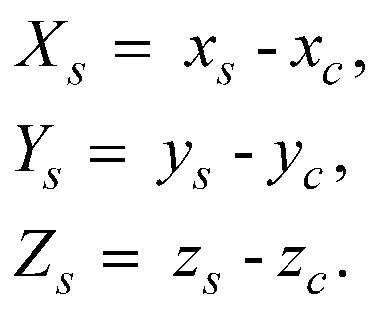
The axis are rotated using the transformation
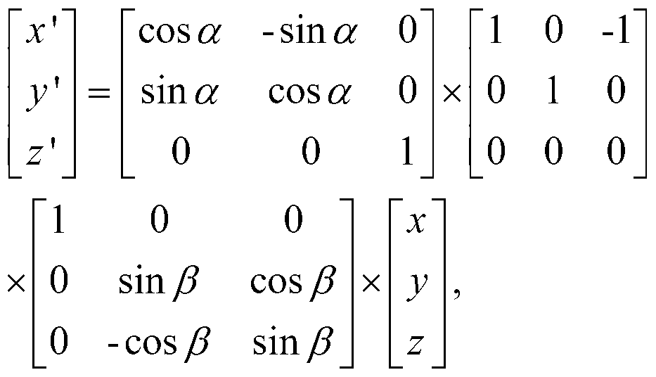


where, the order of the axis rotation is first a rotation about the z-axis, then a rotation about the new y-axis. After this transformation of axes, the problem reduces to the standard form.
Applying Monte-Carlo method to the standard form
A Monte-Carlo method of simulation is a computational algorithm which relies on repeated random sampling to solve a problem at hand. This method is most useful for obtaining numerical solutions to problems which are infeasible or too complicated to solve analytically. It is restricted only to those computations in which random number are used to obtain solutions of problems which are inherently deterministic [20]. There is no fixed way of performing Monte-Carlo simulation but the basic pattern of the method is as follows:
- Define a domain of possible inputs.
- Generate inputs randomly from the domain, and perform a deterministic computation on them.
- Aggregate the results of the individual computations into the final result.
Using this, first a point is generated inside/on the sphere. Then, it is verified whether the point lies in the section of the cone or not. The first two steps are repeated k (very large) number of times. Finally, the fraction of intercepted volume is computed by finding out the ratio of the number of points found inside/on the cone section to the number of points generated (k).
Step 1: generation of the points inside the sphere
Let (xs,ys,zs) be the coordinates of the centre of the sphere with radius r, and let rn be any uniform random number. Any random point (x,y,z) in the sphere is generated using the following equations:
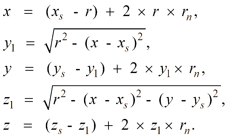
Step 2: constraints of the cone section
If γ and δ be the horizontal and the vertical beam width of the radar and R are the distance of the radar to the tracking point, then the semi-major axis (a) and semi-minor axes (b) of the base-ellipse are given by:
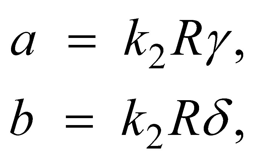
where k2=106 ft/NM [2] and h=R is the height of the elliptic cone, whose equation is given by [21]
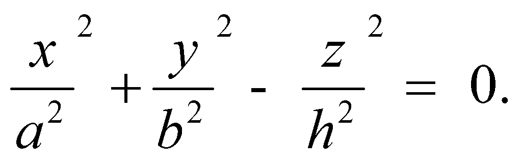
Let hs be the residual height of the section of the cone, this is found out by using the pulse width of the radar beam hs=k1τ, where k1=500 ft/µs [2]. To determine whether any point (x,y,z) on the sphere is in the section of the cone; the inequalities:
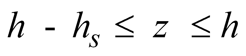
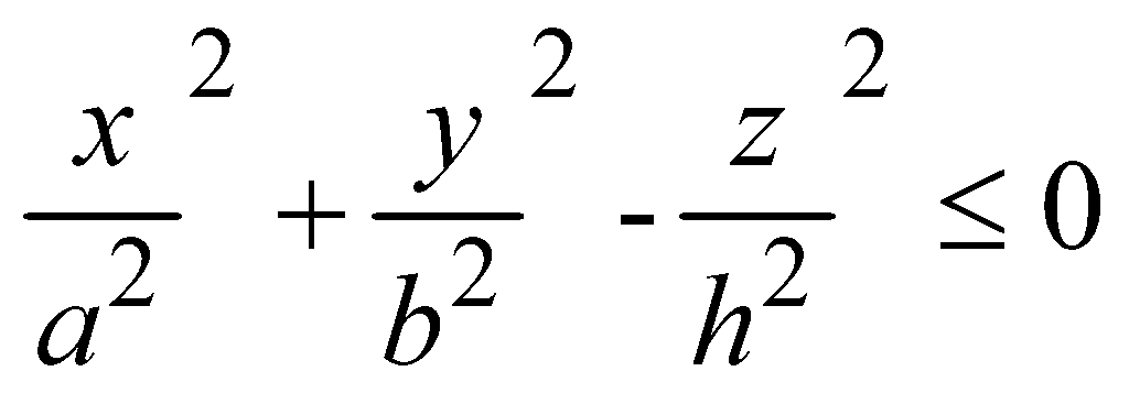
have to be tested against the values of (x,y,z). If both of these inequalities hold, then the point lies inside/on the section of the cone.
Step 3: calculation of intercepted volume
Repeating steps 2 and 3, k number of times, the number of points lying within the section of the cone is obtained. The fraction of the sphere volume is computed by finding the ratio of the number of points found inside/on the cone to the total number of points generated.
The value of this parameter k is very important for the accuracy of the solution. Large values of k results in more accurate solutions but it increases the simulation time. Hence, an optimum value of k is to be calculated. For finding a suitable value of k: say if are the results of k trials and:
are the mean and variance respectively.

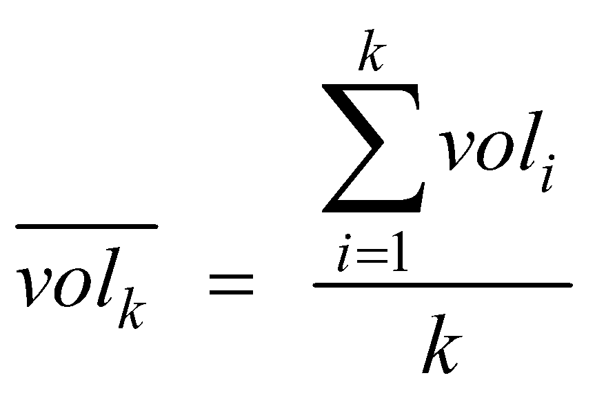
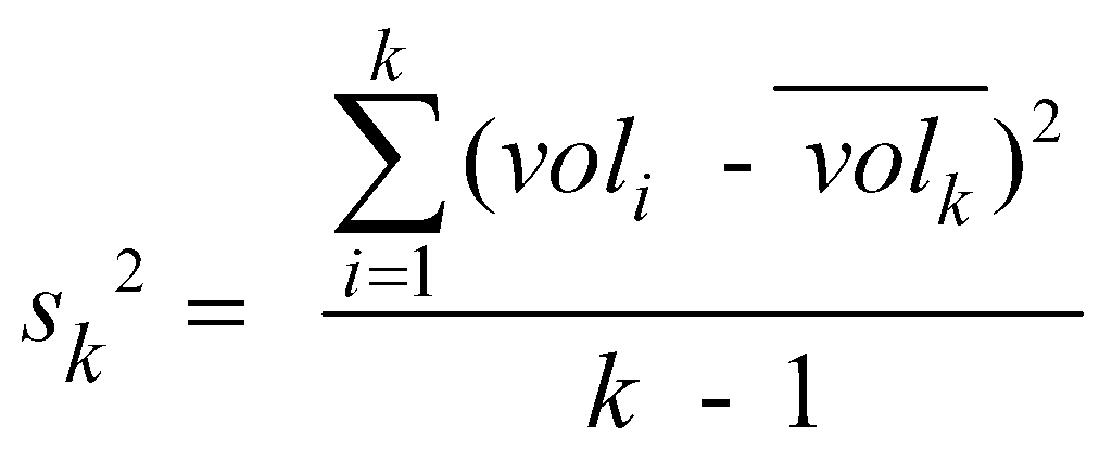
Then, by the law of large numbers, for a large k:
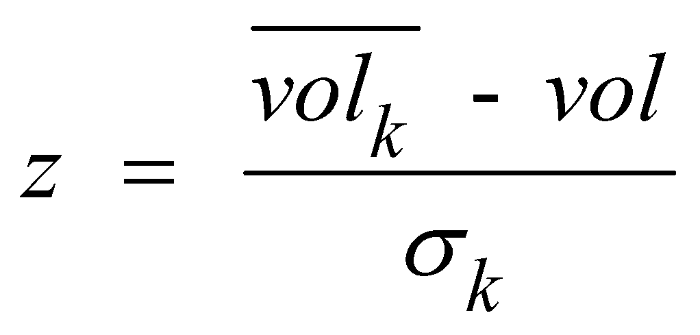
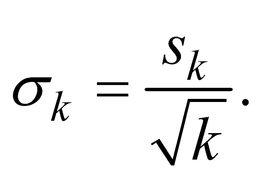
is a standard normal variable, where:
Suppose, solution is needed with 95% confidence level then z=1.96 (using the standard normal curve). The value of k must be so chosen that the inequality
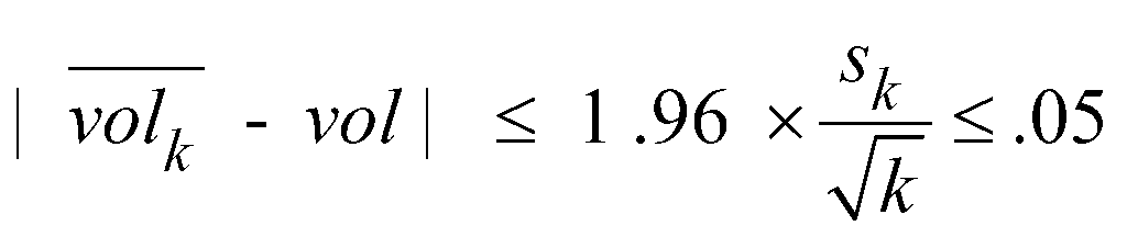
is satisfied [22].
Validation of the proposed technique
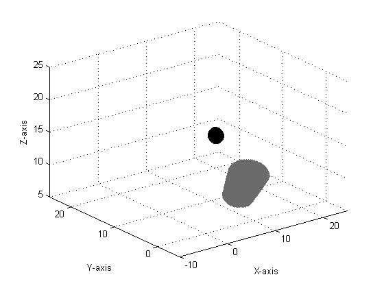
For the purpose of validation, this technique has been implemented in MATLAB and the fraction of the intercepted volume has been estimated for a number of cases. Different cases have been considered by changing the position of the sphere and the orientation of the cone section. The angles made at the vertex by the major and minor axis of the elliptic cone section and its height are taken as 10°, 7°, and 5 units respectively. The radius of the sphere is taken as 1 unit and the vertex of the cone has been kept fixed at the origin.
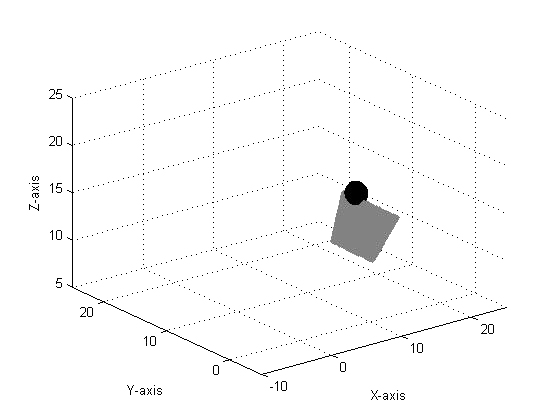
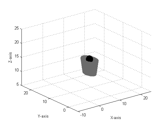
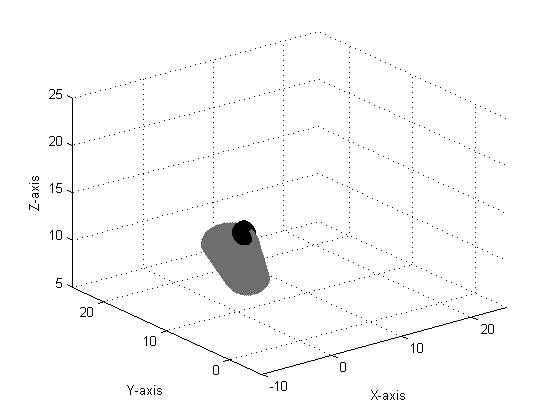
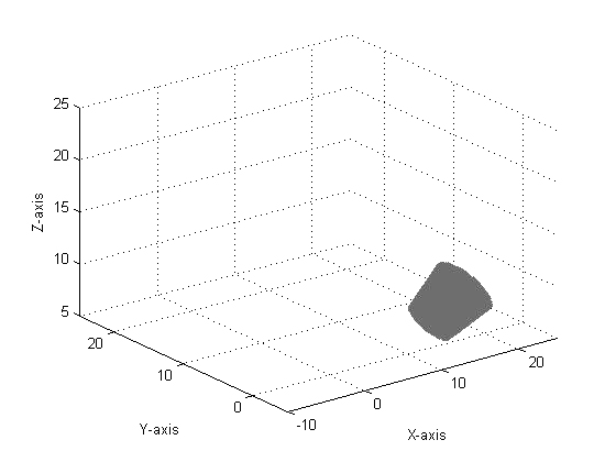
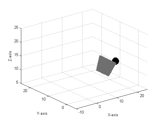
Six different cases have been considered. The position of the sphere, the azimuth and elevation angle of the cone section for each case has been shown in Table 1. All these cases have been graphically shown from Figures 4 to 9 respectively. Comparison of the results obtained using the proposed technique and by analytical computation for each of these cases has been shown in Table 2. It can be observed that the estimated values are either equal or very close to analytically computed values.
| Case No. | Centre of the sphere | Azimuth of the cone section | Elevation of the cone section |
|---|---|---|---|
| I | (20, 20 ,10) | 0° | 60° |
| II | (8, 0, 19) | 90° | 60° |
| III | (0, 0, 20) | 90° | 90° |
| IV | (−8, 0, 18) | 90° | 120° |
| V | (15, 0, 9) | 90° | 30° |
| VI | (12, −2, 17) | 90° | 60° |
Application of the proposed technique
A scenario consisting of a chaff cloud and a point mass missile model tracking a fictitious point (chaff centroid) in the chaff cloud has been simulated to show the application of the proposed technique, with the following assumptions:
- All the dipoles are considered to be randomly oriented.
- The effect of wind in chaff motion has not been considered, only the steady sinking of chaff cloud has been considered.
- The scenario has been simulated only within a short range of 300m.
Estimation of the chaff cloud RCS has been done using the closed form of chaff cloud RCS estimation considering the scattering, bird nesting, and polarization properties of the dipoles [23]:

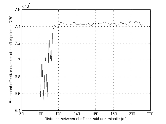
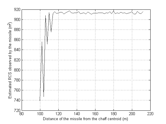
where, Aθφ is the area of the radar beam associated with the RRC of interest if the chaff cloud is larger than the RRC. AC is the projected area of the cloud normal to antenna axis if chaff cloud is smaller than RRC. The chaff cloud of radius 15m is considered at (300,0,65)m sinking with rate 5 m/s. The number of chaff dipoles in the payload is taken to be 767000.The initial position of the missile is taken to be at (0,0,60)m tracking the chaff centroid at (314,0,55) (this is assumed to be different from the chaff centre as it is usually the case due to the presence of the target) with velocity 80 m/sec. The estimated effective number of dipoles and the chaff RCS has been observed at different distances of the missile from the chaff centroid shown in Figure 10 and Figure 11 respectively.
| Case No. | Estimated Values | Analytically Computed Values |
|---|---|---|
| I | 0 | 0 |
| II | 0.0467 | 0.0464 |
| III | 0.4998 | 0.5 |
| IV | 0.5838 | 0.5768 |
| V | 1 | 1 |
| VI | 0.0196 | 0.0211 |
It can be observed from these figures that the effective number of chaff dipoles and chaff RCS are dynamically changing and these changes are highly erratic at shorter distances due to the smaller size of RRC than the chaff cloud and their relative motion. Hence, using this technique the realistic effect in chaff missile engagement can be captured in simulation.
Conclusion
The classical technique for estimation of number of effective chaff dipoles caters only for the changing volume of the chaff cloud and the RRC of the missile seeker. However, the positions and dimensions of the systems change dynamically. In order to estimate the effective number of chaff dipoles for such dynamic scenarios, a technique has been proposed based upon the Monte-Carlo simulation method. For validation purpose a comparative study of the results obtained by using the suggested technique and analytical computation has been done. Furthermore, to show the application potential of the proposed technique a scenario consisting of a point mass missile model tracking a fictitious point in the chaff cloud has been simulated. From the results it has been observed that the proposed technique is able to capture the effects of the realistic engagement in simulation.
Acknowledgement
The authors would like to thank Sh. H. V. Srinivasa Rao Director, Institute for Systems Studies and Analyses for his kind permission to publish this work. The authors would also like to thank Sh. Debasis Dutta and Smt. Aparna Malhotra for their suggestions and support.
References
[1] P. Elecktronikindstrier, Chaff for Ships: Operational Considerations, International Countermeasures Handbook (ICH), 1981.
[2] F.A.D. Macedo, “Analysis of Chaff Cloud RCS applying Fuzzy Calculus”, IEEE Microwave and Optoelectronics International Conference, pp. 724−728, 1997.
[3] R.H. Macfadzean, Surface-Based Air Defence System Analysis, 1992.
[4] H. Saidi, G.H. Askari, J. Akhlaghi, and H.M. Sadeghi, “An Antichaff Technique for Radar Tracking”, IEEE Radar Conference, EURAD, pp. 407−410, 2005.
[5] R.G. Wickliff and R.J. Garbacz, “The Average Backscattering Cross Section of Clouds of Randomized Resonant Dipoles”, IEEE Transactions on Antenna and Propagation, pp. 503−505, 1974.
[6] A.D. Katsicogiannis, Optimal Estimation of Target in Clutter (Chaff) from Radar, Master’s Thesis: AD-A164200, Naval Postgraduate School, 1985.
[7] S.W. Marcus, “Dynamics and Radar Cross Section Density of Chaff Clouds”, IEEE Transactions on Aerospace and Electronic Systems, Vol. 40, No. 1, pp. 93−102, 2004.
[8] X. Wu, Q. Shen, and T. Long, “Chaff Jamming Effect to Radar and Math Model Building”, IEEE Radar International Conference, CIE-06, pp. 324−328, 2006.
[9] W. Zhang, G. Wang, Y. Zeng, and L. Wang, “The Verification and Analysis of Chaff Clouds RCS Distribution Model”, IEEE Antennas and EM Theory International Symposium, pp. 1220−1223, 2008.
[10] S.L. Borison, Statistics of the Radar Cross Section of a Volume of Chaff, Technical Report: 612887, Massachusetts Institute of Technology Lincoln Laboratory, 10 February 1965.
[11] J. Brunk, D. Mihora, and P. Jaffe, Chaff Aerodynamics, Technical Report: AFAL-TR-75-81, Alpha Research, Incorporated, Air Force Avionics Laboratory, November 1975.
[12] P.K Mitchell and R.H Short, Chaff: Basic Characteristics and Applications Detailed, International Countermeasure Handbook (ICH), 1980.
[13] R.H. Short, Chaff: Conceptions and Misconceptions, International Countermeasure Handbook (ICH), 1985.
[14] H.F. Eustace (ed), Aircraft Chaff: Centroid Effects, International Countermeasure Handbook (ICH), 1981.
[15] B.C.F. Butters, “Chaff”, IEE Proceedings Communication Radar and Signal Processing, Vol. 129, No 3, pp. 197–201, June 1982.
[16] P. Pouliguen, O. Bechu, and J.L. Pinchot, “Simulation of Chaff Cloud Radar Cross Section”, IEEE Antennas and Propagation Society International Symposium, Vol-3A, pp. 80−83, 2005.
[17] S.W. Marcus, “The RCS of Large Dense Chaff Clouds”, IEEE Antennas and Propagation Society International Symposium, pp. 3251−3254, 2006.
[18] M. Mahanaffey, Electrical Fundamentals of Countermeasure Chaff, International Countermeasure Handbook (ICH), 1976.
[19] W.E. Byerly, Elements of Integral Calculus with a Key to the Solution of Differential Equations and a Short Table of Integrals, G.E. Stechert and Co., New York, 1941.
[20] N. Deo, System Simulation with Digital Computing, Prentice Hall of India, New Delhi, 2001.
[21] B.S. Grewal, Higher Engineering Mathematics, Khanna Publishers, Delhi, 1975.
[22] N.K. Jaiswal, Military Operation Research, Quantitative Decision Making, Kluwer Academic Publishers, 2003.
[23] P.K Mitchell and R.H Short, How to Plan a Chaff Corridor, International Countermeasure Handbook (ICH), 1979.