
Volume 12, Number 2, July 2009
Digital Ship Internet Protocol Backbone Modelling And Validation
- 1 Land and Joint Systems, Thales Australia, Garden Island, NSW 2011.
Abstract
Next-generation Network Centric Warfare (NCW) [1] foresees naval platforms running unified Internet Protocol (IP) networks capable of running different applications on the same backbone. To promote this NCW concept, Thales Australia has proposed a digital ship local area network (LAN) architecture called the Ship Unified Network IP for Communications Ship (SUNI/CS). A small-scale prototype of this SUNI/CS network has been constructed in Thales Australia's Network Enabled Warfare Laboratory (NEWLab). To mitigate the technical risks of a large-scale deployable digital ship LAN, the network performance and capacity needs to be understood before deployment. Clearly it is impractical to build a full-scale digital ship LAN in a laboratory environment. To overcome this, modelling and simulation of network performance using a discrete event simulator such as OPNET is required. As the first step in modelling a large-scale deployable digital ship LAN, a benchmark study has been conducted to validate the OPNET models against real-life measurements on the SUNI/CS network. In this study, packet delay and throughput were simulated in OPNET and measured on SUNI/CS. A comparison of these results showed the simulated OPNET model accurately matched the measured SUNI/CS results. This study paved the way for future efforts in network capacity and performance measurement on a real-scale digital ship LAN OPNET model.
Introduction
The future Network Centric Warfare (NCW) [1] platform shows a unified Internet Protocol (IP) network in naval arenas where different applications such as file transfer, printing, web browsing, emailing, database access, video conferencing, voice over IP (VoIP), sensor grid feeds, security and surveillance camera streams all run on the same IP backbone. Different applications may have different Quality-of-Service (QoS) requirements. To enable NCW, Thales Australia has proposed a digital ship local area network (LAN) architecture called the Ship Unified Network IP for Communications Ship (SUNI/CS). Inside Thales Australia’s Network Enabled Warfare Laboratory (NEWLab), a prototype of this SUNI/CS network has been constructed as shown in Figure 1.
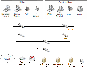
The SUNI/CS network backbone was assembled using six Alcatel-Lucent OmniSwitch 6850 switches (10/100/1000 Mbps) connected in a redundant topology. This redundancy provides high network reliability and availability against link and device failures. To generate traffic on the network, seven PCs, one voice terminal, one VoIP phone and three IP cameras were connected. Different military applications have been installed including Llama/Cheetah, Mercury military messaging, integrated combat management system (ICMS), and simulated sonar and sensor input. Standard applications have also been installed such as FTP clients and servers, HTTP servers and web browsers, databases, conference servers, media players and soft phones. Alcatel-Lucent OmniVista and VitalSuite were also used for network management and performance indication.
This SUNI/CS network constructed in NEWLab is small scale compared to a typical Air Warfare Destroyer (AWD) or ANZAC ship. These could have 50−70 switches, 60−120 voice terminals and IP phones, 200+ workstations and consoles, 20−50 servers and a large number of cameras and sensors. A network of this scale would have many devices communicating simultaneously requiring a network backbone of sufficient capacity. To mitigate the risk of network bottlenecks on a real deployed network of this scale, it is important to understand the backbone network capacity. It is also essential to understand the bandwidth requirements of different applications in a real operational environment. While it is impractical to build such a large-scale network in a test environment, OPNET modelling allows these studies to be carried out on a large-scale simulated network.
Before any modelling of a full scale ship LAN, the network performance results such as packet delay and throughput need to be verified. To do this, the aim is to simulate a smaller-scale SUNI/CS network which is able to be verified and calibrated if necessary in OPNET against real-life measurements on the physical SUNI/CS network. This will ensure that the OPNET models can accurately simulate real network performance. After this verification and validation, the OPNET models will be assured to simulate a real digital ship LAN. A complete description of our study has been provided in our technical report [2]. Interested readers can refer to this for more details.
Experiment and simulation settings
The configuration of the SUNI/CS network and OPNET modelled network were configured to provide as close a match as possible between the simulated and measured results. The three areas of experiment and analysis covered network topology and spanning tree [3], packet delay, and network throughput.
Network topology and spanning tree
2.1.1 SUNI/CS Experiment Settings
Figure 2 shows the backbone network topology used in the spanning tree and network throughput experiments. Packet delay experiments use a different cascaded topology which will be described in Section 2.2.1.
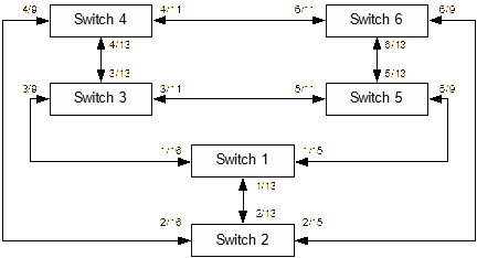
The 'X/Y' notation denotes port 'Y' of switch 'X'. One of the important parameter settings for the SUNI/CS network is the transmission speed of each switch port. This speed can be set to different Ethernet speeds using the Alcatel Operating System (AOS) Command Line Interface (CLI). For example, the following command [4] sets the speed of Switch 6, port 11 to 10 Mbps.
→ interfaces 6/11 speed 10
Besides transmission speed, switch priority is another important parameter to set because it influences the formation of the spanning tree. Switches send Bridge Protocol Data Units (BPDUs) to communicate with each other to form a loop free spanning tree topology. In these experiments, Switch 1 is set to the highest priority (with lowest number), Switch 2 to the second highest priority and so on. The industry standard Rapid Spanning Tree Protocol (RSTP, IEEE 802.1w) was used on all switches.
2.1.2 OPNET Simulation Settings
The network topology used in OPNET was exactly the same as the SUNI/CS network, as shown in Figure 3. The switch model used in the simulation is the OPNET standard 'ethernet32_switch' model [5].
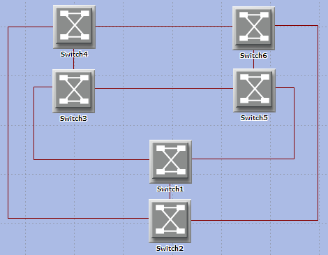
All modelled switch settings were set to match the OmniSwitch 6850 switches used in the SUNI/CS network. However, instead of setting the switch port transmission speed individually, OPNET Ethernet ‘10BaseT’ and ‘100BaseT’ link models were used to connect switches. 10BaseT and 100BaseT represent a full duplex Ethernet connection at 10 Mbps and 100 Mbps respectively. The switch priorities were set to the same values as used in the SUNI/CS experiments. In addition, all OPNET switch models also ran RSTP (IEEE 802.1w) protocol.
Packet delay
2.2.1 SUNI/CS Experimental Settings
Packet delay is difficult to measure using general PCs because it requires the PCs to be synchronised on less than a microsecond scale to conduct accurate measurements. Instead, frame delay can be measured using a SmartBits 600 which is specifically designed for latency measurement [6]. The SmartBits 600 is a network performance analyser (NPA) that has two ports. These two ports are connected to the device(s) under test (DUT) in a transmit/receive loop. It can measure the frame latency through both store-and-forward or cut-through switches. By using one frame as a reference, the NPA can record the time interval using either the last in, first out (LIFO) or first in, first out (FIFO) methods. The LIFO method is used for store and forward switches by measuring the time interval starting when the end of the last bit of the input frame reaches the DUT input port, and ending when the first bit of the output frame is seen on the DUT output port [7]. For bit forwarding (cut-through) devices, the NPA calculates latency using FIFO. The FIFO time interval is between when the end of the first bit of the input frame reaches the DUT input port, and when the first bit of the output frame is seen on the DUT output port [7]. It should be noted that packet delay and frame delay are used interchangeably since the SmartBits 600 uses frames at layer 2, and OPNET uses packets at layer 3.
LIFO packet delay measurement was used across the store-and-forward OmniSwitch 6850 switches. When latency is measured across more than one switch in cascade, this measurement includes processing delay as well as transmission delay. Latency measurement across one switch is effectively measuring only the processing time of the switch. However if two switches are connected in cascade, the measurement will include the delay due to frame transmission from Switch 1 to Switch 2. Figure 4 shows an example of the transmission sequence of a frame across two switches connected in cascade.
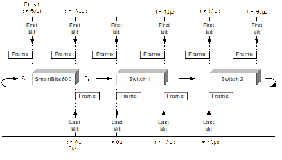
It can be seen that the measured latency using LIFO is 50µs from start time t = 0 µs to finish time t = 50 µs. However, this measured (network) latency not only includes the frame processing time inside both Switch 1 and Switch 2, but also the frame transmission time of Switch 1. Figure 4 shows that the latency in Switch 1 is 10 µs (from t = 0 µs to t = 10 µs) and the latency in Switch 2 is also 10 µs (from t = 40 µs to t = 50 µs). In addition, the transmission time of the frame by Switch 1 is 30 µs (from t = 10 µs to t = 40 µs). The frame propagation delays in the network cables are ignored.
To ensure reliable measurement of latency, SmartBits sends a burst of frames for a pre-set duration to make the DUT establish a link under normal traffic conditions. In the middle of the burst stream, one frame is tagged with an identifying trigger. This frame is timestamped when it is transmitted by SmartBits. This frame then passes through the DUT and is timestamped again when it is received by SmartBits. The latency is then calculated as follows [6].
Latency = Receive Timestamp - Transmit Timestamp
For LIFO latency measurement, the transmit timestamp is made when the last bit of the tagged frame has been transmitted by SmartBits. The receive timestamp is made when the first bit of the tagged frame has been received by SmartBits, as shown in Figure 5. This receive timestamp is made after the seven-byte ‘Start Frame Delimiter’ and one-byte ‘Preamble’ of the standard Ethernet frame.
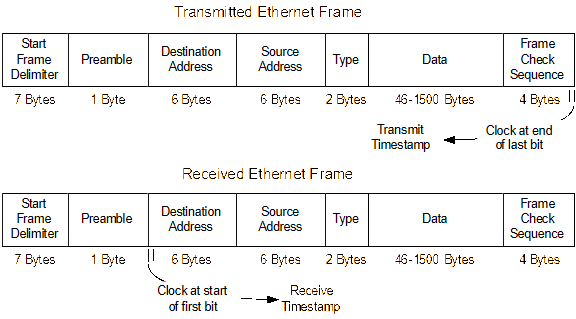
The SmartBits 600 does not measure LIFO latency directly. Instead, it measures the cut-through latency (FIFO) first and then calculates the store-and-forward (LIFO) latency as follows [6]
Store-and-Forward Latency = Cut-through Latency - Frame Bit Time
The ‘Frame Bit Time’ denotes the transmission time of one frame, which is only dependent on bit rate and frame size. However, for the SmartBits measurement to be compatible with OPNET measurement, SmartBits FIFO results need to be used. In comparison studies with OPNET simulations, the SmartBits measurement is regarded as a delay and not exclusively as latency based on OPNET’s convention. This delay comprises the processing time and transmission time of the DUT, whereas latency can be considered as only the processing time. OPNET measures the end-to-end packet delay as the time interval starting when the first bit of the frame is transmitted and ending when the last bit of the frame is received. This is equivalent to first-in-last-out (FILO) if we ignore cable propagation delay. Obviously the SmartBits FIFO measurement is not completely identical with the OPNET FILO measurement. The OPNET measurements will have a time difference of one frame transmission greater than the SmartBits FIFO measurement. The packet delay is measured by connecting SmartBits from one switch up to six switches in cascade. Figure 6 shows an example of the wiring connection for six switches in cascade.
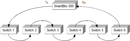
Packet delay was measured using either 10 Mbps or 100 Mbps backbone speeds. All switches and SmartBit transmission ports are set to match the backbone speed. Based on RFC 2544 recommendations [8], delay was measured using frame sizes of 64, 128, 256, 512, 1024, 1280 and 1518 bytes (excluding the seven-byte ‘Start Frame Delimiter’ and 1-byte ‘Preamble’, refer Figure 5). These frame sizes are scaled from the smallest to the largest allowable frame size for Ethernet standard. To achieve proper statistical significance, the average is calculated of 30 repetitions conducted for each experimental combination. The variables are number of switches in cascade, frame size and backbone speed.
2.2.2 OPNET Simulation Settings
Similar to the spanning tree modelling study, the same ‘ethernet32_switch’ model is used. Figure 7 shows a simple topology where two switches are connected in cascade. A sender node is connected to Switch 1 and a receiver node is connected to Switch 2. Both sender and receiver nodes used a standard OPNET ‘ethernet_ip_station’ model [5] with a simple traffic generator sitting above the standard IP layer.
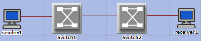
In the simulation, sender node transmits IP traffic to receiver node. The traffic generator process can record and calculate pre-selected statistics such as the traffic sent at sender side, traffic received and packet delay at receiver side. The packet delay was the statistic of interest. The packet generated by the traffic generator process corresponds to the ‘Data’ field of the standard Ethernet frame as shown in Figure 5, but without the IP header. Hence the packet sizes used in the traffic generator process were set to 26, 90, 218, 474, 986, 1242 and 1480 bytes. These packet sizes corresponded to the Media Access Control (MAC) frame sizes used in the SmartBit experiments. For example, the 26 bytes data packet results in 26 bytes + 20 bytes IP header + 18 bytes MAC header and FCS = 64 bytes MAC Frame (refer Figure 5).
| Table 1. Low Traffic Load | ||
|---|---|---|
| Bit Rate (Mbps) | Packet Generation Rate (packet/s) | Packet Inter-Arrival Time (ms) |
| 1.176 | 100 | 10 |
| 2.352 | 200 | 5 |
| 3.528 | 300 | 3.33333 |
| 4.704 | 400 | 2.5 |
| 5.88 | 500 | 2 |
| 7.056 | 600 | 1.66667 |
| 8.232 | 700 | 1.42857 |
| 9.408 | 800 | 1.25 |
| 10.584 | 900 | 1.11111 |
| 11.76 | 1000 | 1 |
| Table 2. High Traffic Load | ||
|---|---|---|
| Bit Rate (Mbps) | Packet Generation Rate (packet/s) | Packet Inter-Arrival Time (ms) |
| 11.76 | 1000 | 1 |
| 23.52 | 2000 | 0.5 |
| 35.28 | 3000 | 0.333333 |
| 47.04 | 4000 | 0.25 |
| 58.8 | 5000 | 0.2 |
| 70.56 | 6000 | 0.166667 |
| 82.32 | 7000 | 0.142857 |
| 94.08 | 8000 | 0.125 |
| 105.84 | 9000 | 0.111111 |
| 117.6 | 10000 | 0.1 |
As mentioned before, OPNET (in fact, the traffic generator process) calculates end-to-end packet delay. This means that the delay is calculated above the IP layer (Network Layer). In contrast, the SmartBit 600 measures frame latency at the MAC Layer. Since OPNET assumes packet transfer across layers has no delay, the layer difference in measurement will not affect experiment results.
One difficulty encountered during the OPNET simulation was setting the Packet Service Rate switch attribute. This attribute specifies the rate at which frames are switched from the switch processor to the appropriate output port. The reciprocal of this attribute represents the frame sojourn time inside the switch. Clearly this sojourn time contributes to the end-to-end packet delay. However, this parameter is not clearly specified in the documents for the Alcatel-Lucent switch. During the SmartBit experimentation, it was found that different transmission rates resulted in different frame sojourn times. Hence the OPNET models were calibrated using the experiment data obtained using the OmniSwitch 6850 switches. Further information is in section 3.2.2.
Network throughput
2.3.1 SUNI/CS Experimental Settings
Network throughput refers to the data transmission rate in bits per second through a communication channel. In the SUNI/CS scenario, a communication channel is the wired connection between two computers across two or more switches. Multiple PCs were connected to the SUNI/CS backbone (as shown in Figure 2) and a simple client/server program called IPERF was used to generate UDP traffic from one node to another. The command to start the IPERF server on a Windows system is as follows.
> iperf.exe -s -u -i 1
---------------------------------------------------
Server listening on UDP port 5001
Receiving 1470 byte datagrams
UDP buffer size: 105 KByte (default)
---------------------------------------------------
where:
- '-s' option denotes this is a server process
- '-u' means this server accepts UDP datagrams
- '-i 1' sets the server to report performance data every second
The default UDP port is 5001 if not specified. The default UDP datagram size is set to 1470 bytes. The following command sends UDP datagrams from client to server,
> iperf.exe -c 192.168.9.4 -u -b 1.176m -t 60
where:
- '-c 192.168.9.4' means to run IPERF in client mode and connect to server with IP address '192.168.9.4' (default port 5001)
- '-u' means this client will send UDP datagrams to the server
- '-b 1.176m' specifies the UDP bit rate to send in Mbits/sec
- '-t 60' sets to run the client process for 60 seconds and then terminate
The 1.176 Mbps bit rate was deliberately selected after examining the IPERF source code. This setting resulted in the UDP packet generation rate being exactly 100 packets/s. This made it easier to set the corresponding parameter in the OPNET models to generate exact traffic load. Note that the throughput measured by IPERF represents the UDP datagram throughput without IP header, MAC header, Ethernet start frame delimiter and preamble (refer Figure 5). In these experiments, a low or high traffic load is selected along with 10 or 100 Mbps backbone Ethernet speed. The low traffic load has packet generation rates from 100 packets/s to 1,000 packets/s in 100 packets/s steps. The high traffic load has packet generation rates from 1,000 packets/s to 10,000 packets/s in 1,000 packets/s steps. This traffic rate remains constant until the end of an experiment. The bit rate for each packet generation rate used in the experiments is listed in Tables 1 and 2. Corresponding ‘Packet Inter-Arrival Time’ values that were used in OPNET simulations are also listed.
2.3.2 OPNET Simulation Settings
Similar to the spanning tree and packet delay simulation, the same OPNET ‘ethernet32_switch’ was used as the switch model and ‘ethernet_ip_station’ as traffic generator. An important attribute for the switch model is the packet buffer size. The default setting for the buffer size of ‘ethernet32_switch’ is infinity. This means that there is no packet drop due to buffer overflows in an ‘ethernet32_switch’ model. However, an OmniSwitch 6850 has a limited 2MB (16 Mbits) packet buffer causing packets to be lost when the buffer is full. To simulate this behaviour, the buffer size in the OPNET switch model was set to the same capacity. The corresponding parameter for buffer size in OPNET is the ‘subqueue’ process interface of the ‘ethernet_mac_v2’ process model. Here the ‘bit capacity’ of ‘subqueue’ to was set to16 Mbits.
The two main attribute settings for the ‘ethernet_ip_station’ are ‘Packet Size’ and ‘Packet Inter-Arrival Time’. The ‘Packet Size’ was set to 1470 bytes which equals the UDP packet size used in the IPERF experiments. OPNET’s ‘Packet Inter-Arrival Time’ equals the reciprocal of the packet generation rate used in IPERF measurements. To generate different traffic loads in OPNET simulations, each packet inter-arrival time from Tables 1 and 2 was used. This traffic load remains constant during an experiment. Using constant packet inter-arrival intervals however caused a problem during two-flow scenario simulations. A two-flow scenario has two sender-receiver pairs in the network. As an example, Figure 8 shows a two-flow scenario where sender 1 sends traffic to receiver 1 and sender 2 sends traffic to receiver 2 simultaneously.
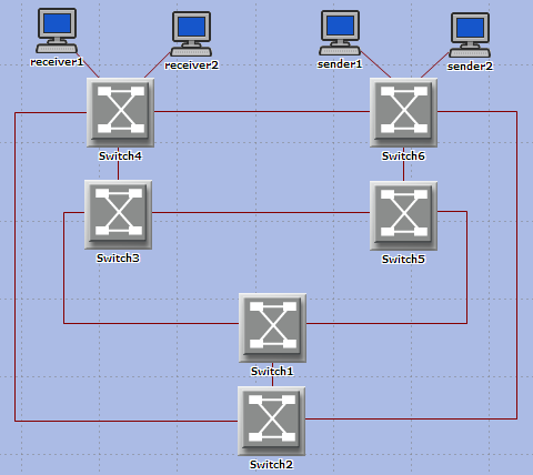
A problem occurs when the link capacity is deliberately saturated by continuously increasing the traffic load. This problem was only exhibited in high traffic scenarios, not low traffic scenarios. This is due to low traffic not causing a buffer overflow unlike high traffic. The symptom of the problem is that one sender’s packets can always pass through while the other sender's packets are continually discarded when the buffer is full. This behaviour did not match with the IPERF experiment results where the two flows equally share the saturated bandwidth.
Since OPNET is a discrete event simulator, it depends on how events are executed one after another. This problem is expressed as a ‘tightly controlled event based discrete event simulation’. Setting the packet inter-arrival time to an exact constant value may result in abnormal behaviour during the simulations that does not match with the IPERF experiment results. This could happen when the buffer of a switch is nearly full, and a packet from sender 1 happens to arrive at a time when the switch module has ‘just’ finished processing and forwarded a packet. This packet from sender 1 is able to be stored on the MAC queue. However, a packet from sender 2 could come at an inopportune time when the switch is still processing a packet and has its buffer full, so this packet from sender 2 is discarded. If the packet inter-arrival time is set to an exact constant value, sender 1’s packets will always arrive at an opportune time while sender 2’s packets will always arrive at an inopportune time. This would cause packets from sender 1 to always be able to be queued, while packets from sender 2 would always be discarded. In contrast, such a tight synchronisation is unlikely to happen on a real switch. There will always be some jitter either in the internal processing of the switch or the inter-arrival time of the packets. In a real life situation, the timing sequence of packet delivery and processing will never remain exactly the same, so even a slight jitter is sufficient to allow sender 2’s packets to be queued. To tide over this problem in OPNET modelling, a very narrow uniform distribution is used instead of the constant distribution of packet inter-arrival time in high traffic simulations. Table 3 shows the packet inter-arrival times with uniform distributions used in high traffic scenarios, in comparison to their corresponding constant value.
| Table 3. Packet Inter-Arrival Time for High Traffic Load | |
|---|---|
| Constant Packet Inter-Arrival Time (second) | Packet Inter-Arrival Time (second) with uniform distribution (min, max) |
| 0.001 | uniform (0.000995,0.001005) |
| 0.0005 | uniform (0.000495, 0.000505) |
| 0.000333333 | uniform (0.000328, 0.000338) |
| 0.00025 | uniform (0.000245, 0.000255) |
| 0.0002 | uniform (0.000195, 0.000205) |
| 0.000166667 | uniform (0.000162, 0.000172) |
| 0.000142857 | uniform (0.000138, 0.000148) |
| 0.000125 | uniform (0.000120, 0.000130) |
| 0.000111111 | uniform (0.000106, 0.000116) |
| 0.0001 | uniform (0.000095, 0.000105) |
Another issue has been identified during OPNET simulation. The ‘ethernet_ip_station’ model in use only generates pure unidirectional flow from one node to another. For example, in Figure 8, sender 1 (sender 2) sends unidirectional flow to receiver 1 (receiver 2), but receiver 1 does not reply with any acknowledgement packet. This causes the filtering database entry in Switch 4 about receiver 1 to not be updated after approximately 30 seconds, and causes it to be removed from the filtering database. At this point, Switch 4 does not know how to reach receiver 1 which makes it broadcast any traffic it receives for receiver 1 through its unblocked ports. This behaviour is different from the IPERF experiments, where receiver 1 periodically sends background traffic to Switch 4. In addition during IPERF experiments, receiver 1 also periodically replies messages to sender 1 in order to report the performance data. This results in the filtering database entry in Switch 4 about receiver 1 being updated periodically, so Switch 4 always knows how to reach receiver 1. To resolve this problem in OPNET modelling, receiver 1 is set to send very light traffic (for example, 1 small size packet for every 10-15 seconds) to sender 1. In this way, Switch 4 can update its filtering database entry for receiver 1 periodically and so Switch 4 no longer sends broadcast packets for receiver 1 through all its unblocked ports. By doing so, the behaviour of OPNET modelling matches the behaviour of IPERF experiments on the SUNI/CS network.
Experiment and simulation results
This section compares and analyses the experiment results using the SUNI/CS network and simulation results using OPNET modelling. It is demonstrated that OPNET models can accurately simulate SUNI/CS network performance. Due to space limitations, only a small part of these results have been included. For a complete description, please refer to [2].
Network topology and spanning tree
3.1.1 Results and Analysis
Table 4 shows the spanning tree information (using AOS CLI ‘show spantree ports’ command) for all six switches shown in Figure 2. FORW means forwarding state, BLK means blocking state, DESG means designed port, ROOT means root port, and ALT means alternate port.
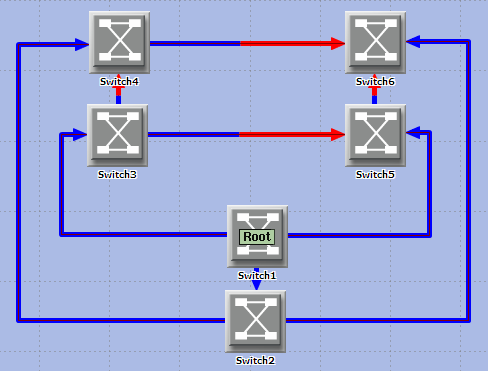
Given Switch 1 (with the highest priority) has been elected as the root switch, all its active ports are designed ports and operate at forwarding state (refer Figure 2). Switch 2 connects to Switch 1 through its root port 2/13, while the other two ports—2/15 and 2/16—are designed ports with forwarding state. Similar to Switch 2, Switch 3 connects to Switch 1 through its root port 3/9 and the other ports—3/11 and 3/13—are designed ports with forwarding state. Switch 4 has a root port 4/9 which connects to Switch 2, a designed port 4/11 which connects to Switch 6, and an alternate port 4/13 which has been blocked by the spanning tree protocol. Similarly, Switch 5 has one root port 5/9, one designed port 5/13 and an alternate blocked port 5/11. Switch 6 has only one root port 6/9 which connects to Switch 2. Both of the other ports, 6/11 and 6/13, have been blocked by the spanning tree protocol.
In addition to the above analysis, Figure 9 shows the resulting spanning tree using Alcatel-Lucent’s OmniVista management software. Note that the figure only shows the links connected to root and designed ports with forwarding state (tree branches), not the links connected to blocked ports. Also note that in Figure 9, Switch 11 (192.168.9.11) is equivalent to Figure 2 Switch 1; Switch 12 (192.168.9.12) is equivalent to Figure 2 Switch 2; and so on.
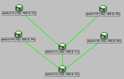
In comparison, Figure 10 shows the resulting spanning tree using OPNET from Figure 3. Clearly, the spanning tree shown in Figure 10 has the same tree topology compared to Figure 9 and Table 4. Figure 10 shows that Switch 1 is the root switch, red arrows point to the blocked ports, and blue arrows show the forwarding path from the root switch (in this case, Switch 1) to all other non-root switches.
Next the operation of the spanning tree protocol is validated with a link failure. The link between Switch 1 → Switch 3 is broken to simulate a link failure in the SUNI/CS network and observe the resulting spanning tree topology. Figure 11 shows the resulting spanning tree topology with the Switch 1 → Switch 3 link failure.
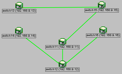
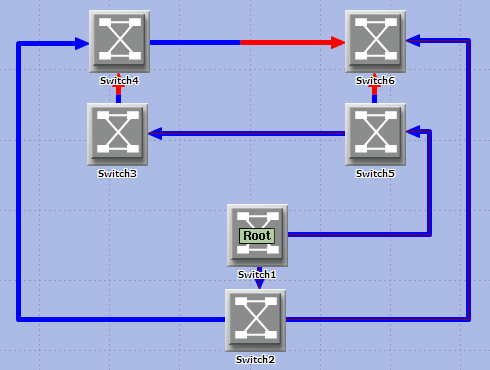
Figure 12 shows the resulting spanning tree topology in OPNET when the link between Switch 1 → Switch 2 is broken. This OPNET model shows the same tree topology as Figure 11.
| Table 4. Spanning Tree Information for All Switches | |||||||
|---|---|---|---|---|---|---|---|
| SW# | Port | Status | Role | SW# | Port | Status | Role |
| SW1 | 1/13 | FORW | DESG | SW2 | 2/13 | FORW | ROOT |
| 1/15 | FORW | DESG | 2/15 | FORW | DESG | ||
| 1/16 | FORW | DESG | 2/16 | FORW | DESG | ||
| SW3 | 3/9 | FORW | ROOT | SW4 | 4/9 | FORW | ROOT |
| 3/11 | FORW | DESG | 4/11 | FORW | DESG | ||
| 3/13 | FORW | DESG | 4/13 | BLK | ALT | ||
| SW5 | 5/9 | FORW | ROOT | SW6 | 6/9 | FORW | ROOT |
| 5/11 | BLK | ALT | 6/11 | BLK | ALT | ||
| 5/13 | FORW | DESG | 6/13 | BLK | ALT |
Packet delay
3.2.1 Results and Analysis
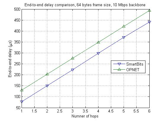
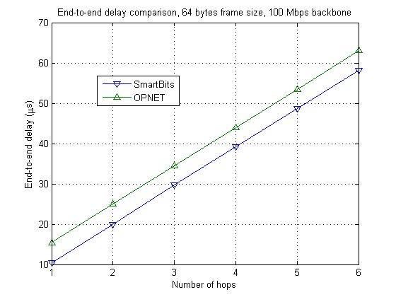
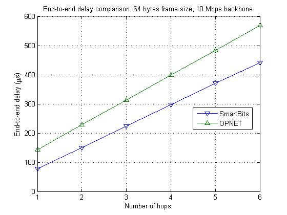
This subsection provides the performance results for the end-to-end packet delay for both the SUNI/CS switched network and OPNET modelling. The experiment results from the SUNI/CS switched network are obtained using the SmartBits 600 with FIFO measuring technique. The OPNET simulations results are collected as an IP traffic end-to-end delay statistic with a measuring technique equivalent to FILO. As mentioned earlier, the end-to-end packet delay has been measured with a different number of switches (from one to six) connected in cascade.
Figures 13 and 14 show the average packet delay (mean value over 30 repetitions) with 64 bytes frame size on 10 Mbps and 100 Mbps backbone respectively. The x-axis represents the number of hops, which is equal to the number of switches connected in cascade (refer to Figure 6).
In contrast, Figures 15 and 16 show the average packet delay with 1518-byte frame size on a 10 Mbps and 100 Mbps backbone respectively.
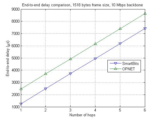
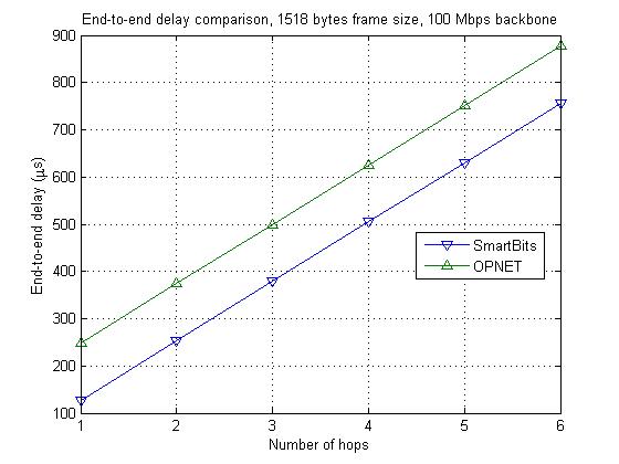
The SmartBits results are lower than the OPNET simulation results due to FIFO and FILO (equivalent) frame delay methods being used respectively. The difference between a FIFO and FILO packet delay measurement equals one frame transmission period. For example, the delay measured for a 1518-byte frame with SmartBits over two switches on 100 Mbps backbone is approximately 252 µs (refer Figure 16), and the OPNET simulation result is approximately 377 µs. This 125 µs difference is equivalent to the transmission period of a 1518-byte frame at 100 Mbps. It can be seen that the two plotted lines (SmartBits and OPNET) on each figure are parallel. This means that the OPNET models accurately simulated the increased delay behaviours of the real switched network as the number of switches connected in cascade is increased.
3.2.2 Lessons Learned
This subsection's results demonstrate that OPNET simulation can accurately simulate the packet delay of the real-life SUNI/CS network. One important lesson learned is that the real switches' experiment results are necessary to calibrate the OPNET models. As mentioned before, the ‘ethernet_ip_station’ model’s attribute ‘Packet Service Rate’ is set to different values based on the experiment results with real switches. Originally, the default setting of this attribute was kept but it was soon found that the OPNET simulation results do not match with the experiment results. A corresponding 'Packet Service Rate' needed to be calculated based on the average value measured in the experiments using real switches. Doing this showed that the OPNET simulation results still do not match with the experiment results very well. As an example, Figure 17 shows one of the original simulation results with the 'Packet Service Rate' setting based on the average value calculated from the experiments using real switches. Figure 17 compared to Figure 13 shows that the OPNET simulation results show a slightly quicker increasing trend (with the increasing number of switches in cascade) than the SmartBits experiment results. To make the OPNET models simulate the behaviour of the real switches more accurately, the 'Packet Service Rate' setting was calculated based on the experiment results on real switches and set to 67,098 packets/s for 10 Mbps backbone and 275,435 packets/s for 100 Mbps backbone. Figures 13 to 16 show that, after the calibration, OPNET simulations model the packet delay with constant difference to real-life measurement. To achieve accurate simulation, the OPNET packet service rate needs to be calibrated based on the performance of real network devices to obtain accurate model behaviours.
Network throughput
3.3.1 Results and Analysis
In both the SUNI/CS network experiments and OPNET simulations, throughput measurements were done using senders transmitting UDP packets. The throughput was measured at the receiving ends.
In all experiments, senders and receivers are deliberately connected around Switch 3, Switch 4, Switch 5, and Switch 6 (refer Figure 3). This is because all blocked ports are around these four switches (refer Figure 10). Network traffic is now forced to pass through multiple hops instead of a single hop. This will generate possible contentions and congestions in the intermediate switches. For example, traffic from sender 1 to receiver 1 in Figure 8 cannot be delivered through the Switch 6→Switch 4 link because the port at Switch 6 has been blocked by the spanning tree protocol. Traffic now has to go through Switch 6 designed port (forwarding port) to be delivered to the end receiver. The generated traffic loads for each sender are based on the packet generation rates from Tables 1 and 2. Due to space limitations, only the results for two two-flow cases are presented, where each case has a different configuration of senders and receivers.
Case 1 scenario uses the sender/receiver topology shown in Figure 8. This scenario has a resulting spanning tree topology shown in Figure 10.
Figures 18 and 19 represent the throughput comparison with low traffic on 10 Mbps backbone, where ‘Receiver1 (IPERF)’ denotes the IPERF measurements and ‘Receiver1 (OPNET)’ denotes the throughput results simulated in OPNET. The offered load for both sender 1 and sender 2 scales from 100 packets/s to 1,000 packets/s.
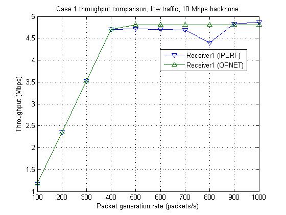
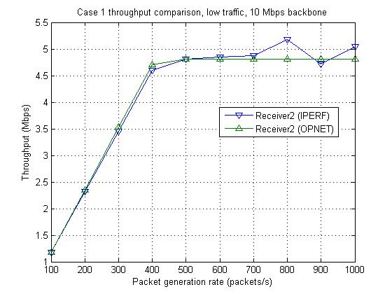
Both IPERF experiments and OPNET simulation results closely match each other when the packet generation rate is lower than 400 packet/s. When the packet generation rate exceeds 400 packet/s (for both senders), the network starts to saturate. These two flows are now following a similar route. Using Figure 8:
Sender1 → Switch6 → Switch2 → Switch4 → Receiver1
Sender2 → Switch6 → Switch2 → Switch4 → Receiver2
This behaviour causes the two flows to interfere with each other. The combined effect is that each flow can only achieve an average of 4.7 Mbps throughput because the backbone bandwidth is set to 10 Mbps. It is also observable that there are some fluctuations of the throughput in the IPERF experiments when the network is saturated (eg at 800 packet/s). This could be caused by the inconsistent operation of real hardware in a saturated environment. For example, some background processes may influence the transmission rate of the UDP datagram. However, it is also observable that while receiver 1 achieves a slightly lower throughput at 800 packet/s, receiver 2 achieves a slightly higher throughput. Overall, the average throughput across both routes is still the same, for example 4.7 Mbps for each flow. In comparison, OPNET simulations run in a much more deterministic environment without the influence of background processes. These simulation results fluctuate less and the plotted throughput shows no fluctuation, even when the network is saturated.
For comparison, low traffic SUNI/CS experiments and OPNET simulations were done on a 100 Mbps backbone. The plotted figures show that lines almost overlapped with each other. This shows that when the generated traffic is well below the network capacity, OPNET simulation results can match the real network performance perfectly. Refer to [2] for these results.
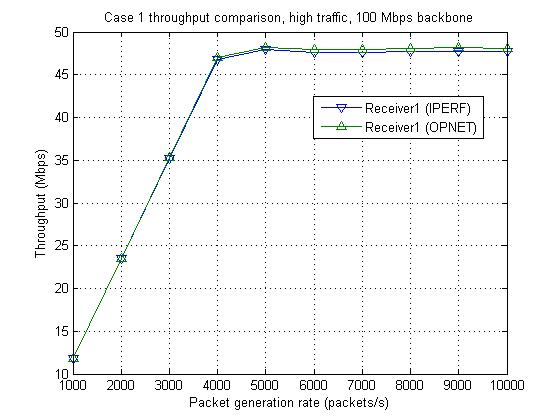
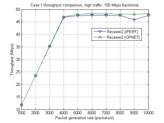
Figures 20 and 21 show the throughput comparison with high traffic on 100 Mbps backbone for Case 1. The figures show a similar trend to Figures 18 and 19, where the network is saturated when the packet generation rate (for both senders) exceeds 4,000 packets/s. The OPNET simulation results match the IPERF experiment results perfectly when the packet generation rate is less than 4000 packets/s, and with only minor fluctuations above this rate when the network is saturated.
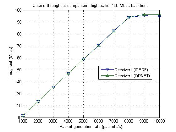
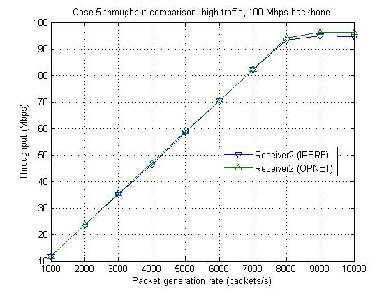
As a second case to consider, Case 5 (original case name from [2]) shows a different two-flow configuration. Similar to Case 1, IPERF experiments and OPNET simulations are carried out with low traffic on a 10 Mbps backbone, low traffic on a 100 Mbps backbone, and high traffic on a 100 Mbps backbone.
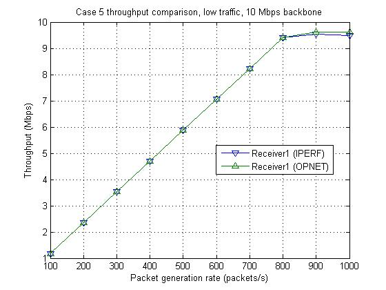
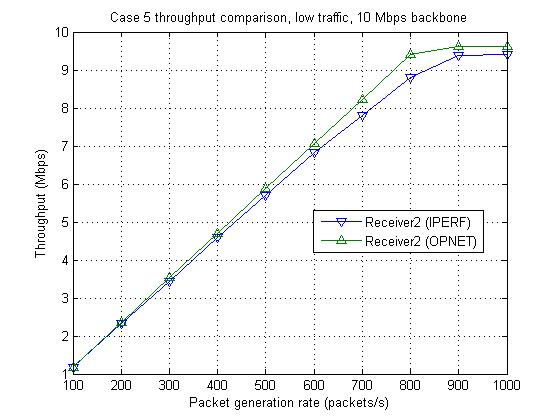
The throughput comparison with low traffic on a 10 Mbps backbone is shown in Figures 23 and 24. The OPNET simulation results match with IPERF experiment results reasonably well, although receiver 2 using IPERF achieves a slight lower throughput than OPNET simulation results. An interesting observation is that the network saturates when the packet generation rate reaches 800 packets/s, with a maximum throughput of approximately 9.6 Mbps for both flows. This is different to Case 1 where network saturation occurs when packet generation reaches 400 packets/s, and throughput approximately 4.7 Mbps for both flows. This implies that there is no interference between the two flows, and hence they both achieve higher throughput than Case 1. In-depth analysis reveals that the two flows follow the following routes:
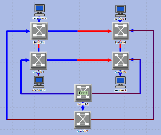
Sender1 → Switch6 → Switch2 → Switch1 → Switch3 → Receiver1
Sender2 → Switch5 → Switch1 → Switch2 → Switch4 → Receiver2
Both flows pass through the Switch 1 → Switch 2 link, but each from an opposite direction. Since Switch 1 → Switch 2 is a duplex link, these two flows do not interfere with each other.
As with Case 1, low traffic on the 100 Mbps backbone shows that the OPNET models match the real network performance perfectly with overlapped lines. Refer to [2] for these results.
The throughput comparisons in Figures 25 and 26 are with high traffic on a 100 Mbps backbone for Case 5. The OPNET simulation results match with the IPERF experiment results reasonably well, even when the network is saturated. Similar to the trend in Figures 23 and 24, the network saturates when the packet generation rate exceeds 8000 packets/s. This is different from Case 1, again due to opposite instead of same direction flow across the Switch 1 → Switch 2 link.
3.3.2 Lessons Learned
This subsection's results demonstrate that the OPNET modelling configuration used can accurately simulate real network throughput performance. By conducting experiments and simulations with low traffic on a 10 Mbps backbone, low traffic on a 100 Mbps backbone, and high traffic on a 100 Mbps backbone, it can be concluded that the OPNET models scale well in simulating real network packet delay and throughput.
One lesson learned is that different combinations of application configurations, and the underlining spanning tree topology, could result in different network performance. For example, a sender/receiver pair connected to Switch 4 and Switch 6 (Figure 8) cannot communicate directly through the Switch 4 → Switch 6 link. This is due to the resulting spanning tree topology blocking this link, although a cable does exist between the two switches. Instead, traffic is diverted through an intermediate Switch 2 to reach the final destination. However, if either the sender or the receiver can be connected to Switch 2, the network traffic can be reduced since Switch 2 and Switch 4 can communicate directly. This avoids the need for an intermediate switch, and eliminates the extra hop that would be introduced. On the other hand, re-organising the spanning tree topology by changing switch priority can also achieve a similar objective. For example, if either Switch 4 or Switch 6 is changed to be the root switch, the link between Switch 4 and Switch 6 will become active. Now the sender/receiver pair connected to Switches 4 and 6 will be able to communicate directly.
It is conceivable that an optimised combination of both application configuration and underlining spanning tree topology could maximise network throughput and balance network utilisation. This is a complex network optimisation problem, especially when the network becomes large. It requires careful flow analysis, traffic engineering and network optimisation techniques—and needs extensive research and development effort.
Concluding remarks and future work
This paper presents a benchmark study to validate the OPNET models against the SUNI/CS network constructed using six Alcatel-Lucent OmniSwitch 6850 switches. It has been demonstrated that configured OPNET models can simulate real network performance accurately. This study also demonstrates that OPNET modelling scales well by comparing SUNI/CS experiment results with OPNET simulation results. Packet delay has been validated across a range of switches connected in cascade, using varying bit rate and frame size. Throughput has also been validated across seven different two-flow scenarios and one single-flow scenario. Each scenario consisted of a different spanning tree topology, packet rate and sender/receiver pair location. A complete description of all the results can be found in [2]. With the OPNET models validated, these simulated models can now be extended to accurately simulate a real digital ship LAN. Extensive simulation and analysis of network traffic and the performance of different user applications can now be carried out on these simulated models.
Acknowledgements
The authors would like to thank Janice McLeod for her extensive assistance proof reading and editing this paper. We would also like to thank Paul Feighan and Darren Milne for their valuable feedback.
References
[1] Network Centric Warfare (NCW) Roadmap, Australian Government, Department of Defence, 2007.
[2] M. Liu, O. Gruber, SUNI/CS Digital Ship IP Backbone Benchmark Study, Technical Report, June 2008.
[3] P. Radia, “An Algorithm for Distributed Computation of a Spanning Tree in an Extended LAN”, ACM SIGCOMM Computer Communication Review, 1985, 15 (4), pp. 44–53.
[4] OmniSwitch 6800 Series, OmniSwitch 6850 Series, OmniSwitch 9000 Series, Network Configuration Guide, Alcatel-Lucent.
[5] OPNET documentation, OPNET Ltd.
[6] SmartBit 600 Smart Applications User Guide, Version 2.50, Spirent Communications, January 2002.
[7] RFC 1242—Benchmarking Terminology for Network Interconnection Devices, July 1991.
[8] RFC 2544—Benchmarking Methodology for Network Interconnect Devices, March 1999.