RF Propagation Environment Awareness (RPEA) For Smart Mobile Ad-Hoc Networks

Introduction

A satisfactory solution for the provision of radio-frequency connectivity for man-portable and vehicular network stations in urban canyon environments remains to be proven. Urban canyons are characterised by significant shadowing problems, which can result in poor propagation where building structures produce large attenuation for the wavelengths of interest.

From a propagation geometry perspective, the best strategy to date remains that of positioning an airborne or satellite relay station at the geometrical zenith for the urban area of interest (Figure 1). This strategy is potentially very expensive, and may be infeasible using satellites for geographical areas at latitudes other than equatorial.

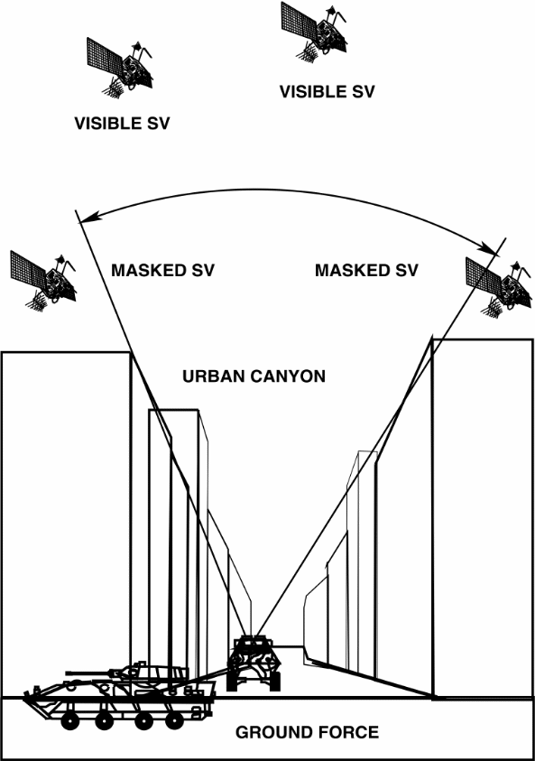
In a civilian context, propagation issues within urban environments can be addressed with the addition of extra network infrastructure, such as the installation of taller masts on base stations, and/or higher power output and higher gain antennas. In an operational military environment, however, this solution is typically infeasible, due to the likelihood of fixed infrastructure being subjected to attack. Deployable elevating or telescoping masts, often employed in military search radar installations, typically present problems with size and weight and thus do not present a good solution for the general case.

This paper introduces an alternate strategy to address this problem, utilising 'smart' ad hoc, or self forming and self healing networks, which are capable of storing and exploiting local propagation geometry information. When used in conjunction with node movement tracking and prediction, this information yields the ability to predict future states of network connections. This in turn provides for a variety of optimisations in network behaviour.

A geographic information system (GIS) database of the local urban topography could be employed to produce local propagation geometry information. However, such systems typically do not address the problem of building structure propagation losses. Consequently, the propagation loss model produced from such a database could yield either unreasonably optimistic or pessimistic results.

Our approach to this problem is much more empirical, and entails exploitation of prior experience operating in the region of interest, to construct over time a database of signal loss measurements. This collection of recorded data is then used to construct and subsequently update an empirical model of the loss environment specific to the local urban topography. The model can be distributed across all network participants, or stored at one or more designated central locations.

This paper explores the principles of RF Propagation Environment Awareness (RPEA) and examines its utility in urban environments.

The following section provides an overview of environmental awareness with respect to ad hoc networking; the section entitled ‘Learning about RF environments’ discusses possible techniques to form an empirical model of local propagation geometry; the ‘Utility’ section investigates factors related to the effectiveness of environmental awareness, and ‘Conclusion’ summarises and describes future research opportunities.

Environmental awareness

Wireless ad hoc networks offer a decentralised, scalable and often relatively inexpensive connectivity solution. Participants co-operatively route traffic through the network, removing the requirement for fixed infrastructure [1−3]. In a civilian context, community networks allow local connections to take place, without requiring a centralised provider. In a military operations context, ad hoc networks provide an inexpensive and rapidly deployable solution for connectivity of man-portable and vehicular network stations.

Mobile ad hoc networks (MANETs) introduce a new set of challenges [4]. Network topologies that include mobile nodes are highly dynamic: peer-to-peer wireless links are formed and broken as nodes move around in the environment.

Some optimisation can be obtained by using information about the geographical properties of the network [5−7]. Location information can be provided a number of ways, including infrared sensors and emitters for indoor networks and radios using time difference of arrival (TDOA) or angle of arrival (AOA) techniques to calculate position [8], [9]. Particularly popular mechanisms for providing location information are Global Navigation Satellite Systems (GNSS), such as the US Global Positioning System (GPS) [10,11].

Use of location information in MANETs allows for various enhancements, such as bounding the search area when performing route discovery optimisations [5], and simplifying routing functions by forming geography-based hierarchies in the routing tree [7].

The success of location awareness in mobile ad hoc networking reveals that awareness of environmental factors that influence the network, in this case the physical geometry of the network, permits optimization of network performance and Quality of Service (QoS). However, in addition to the geometry of the ad hoc network, the topology of the environment in which a wireless network operates also exerts great influence on network operation.

Dense objects, such as buildings or mountains, attenuate wireless signals. This occurs as energy is absorbed or reflected by objects. Thus, network nodes that would otherwise obtain satisfactory signal levels from peers, may be entirely isolated from the desired signal. Reflection and scattering effects also have a significant effect on radio propagation; constructive interference locally increases signal level, whereas destructive interference impairs it. Signals may comprise many delayed copies of the original signal; a form of interference known as multipath, and manifested most visibly as ghosting on an analogue TV set [12].

Given the impact of local radio propagation geometry, further network optimisation is possible with the aid of additional information about the surrounding environment, as opposed to the use of location alone.

In a MANET, where nodes move around frequently, radio propagation impairments severely impact network reliability, particularly when certain QoS is desired. If network participants are able to predict future signal behaviour, decisions about route acquisition and maintenance can be optimised. Giving mobile nodes warning about impending signal problems would allow the network to take action pre-emptively, to avoid service interruption or severe QoS degradation.

When performing a route selection to form a new end-to-end link, this information can be used to optimise link lifetime. Routes containing nodes that are expected to imminently leave wireless range or move into an area with dense objects lying in the signal's path can be avoided, in favour of routes with more stable intermediate links.

Figure 2 depicts one example given local geometry and current node kinematic behaviours. In Figure 2(a), a network node A is currently communicating with network node D, through an intermediate node B. The dashed circle represents A's radio range. Node B is moving towards the right, a state which can be predicted from prior movement. Without RF Propagation Environment Awareness, nodes A and B are unaware of the building about to block their communications channel (Figure 2(b)). The connection will be severed, and a costly delay introduced while node A finds an alternate route to D.

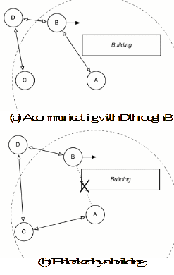
With RF Propagation Environment Awareness, nodes A and B can pre-empt the disconnection, finding an alternate route such that A uses node C as an alternate intermediate node.

Thus, having some knowledge about the propagation environment yields the ability to make better decisions about network operation.

One possible technique involves keeping an RF propagation environment map, where each point on the map represents the instantaneous attenuation at a location in the environment. This map can be built and maintained over time, by incorporating ongoing observations from network participants (as described in the next section). The map can then be used with motion prediction to estimate when shadowing will cause a link to fail, given current node kinematic behaviour.

Note that this does not take into effect any other radio propagation effects such as reflection, scattering, diffraction or interference, and thus will not yield perfect accuracy. A possible avenue for future research involves finding the degree to which disregarding these effects impacts the accuracy of such modelling techniques.

Learning about RF environments

A Smart Mobile Ad-hoc Network with RF Propagation Environment Awareness (RPEA) uses location information and feedback from the physical communication layer to gather information about the local radio propagation environment: by monitoring past behaviour, the network management logic can infer future behaviour. This information, which can be distributed through the network, can be used with movement prediction to predict signal impairment. This provides the ability to pre-emptively form an alternate route for traffic, establish an optimal route, and estimate future path parameters, such as throughput, jitter and lifetime, for QoS functions.

Techniques by which a subject is imaged from many observations of the effect on transmitted energy are widely termed tomography. Traditional tomography, mostly employed in medicine, involves forming an image of a subject, such as a patient's head, from projections taken of the subject [13−15].

Modern technology, such as Computed Tomography (CT), involves taking many single-dimensional projections of the subject, at regular angles (Figure 3), and reconstructing an image from these projections. In CT, emitters transmit X-rays into the subject in a regular geometry, such as parallel lines, or a fan shape. Sensors on the opposite side of the subject record the received energy. Thus, for a single projection, the attenuation is known for each ray. The entire assembly is then rotated, and the process is repeated again, for each projection.

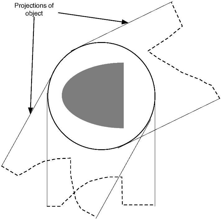
An image of the structure of the subject is then formed using a reconstruction algorithm. A particularly popular algorithm, used in most modern tomographic technology, is known as Filtered Back Projection. This involves taking each projection, filtering it to enhance sharpness, and ‘smearing’ it across the image. That is, the single-dimensional projection is stretched across the image at an angle that corresponds to the angle of projection, making the projection two-dimensional, and combining it with previously processed projections. The result approximates the subject's structure.

Other forms of tomography, such as reflection seismology and ultrasound transmission tomography measure the structure of the subject by observing energy reflected off internal boundaries with differing material densities within the imaged object or volume [16].

In an RPEA context, the detection equipment consists of communicating pairs of network nodes. Given information about received signal power, link distance and receiver/transmitter antenna gain/power/sensitivity, participants can estimate the attenuation effect upon received signals, with some level of accuracy, depending on the hardware, and other factors such as location error, or the magnitude of radio propagation effects other than attenuation. Additionally, network nodes are equipped with a system to provide an estimate of the location of the node, such as a GPS receiver. One technique to make use of this information can be considered a form of tomography. There exist several significant differences between this context and that of traditional tomography. Firstly, the geometry differs greatly (Figure 4). In traditional tomography (Figure 4(a)), the subject is surrounded by detector/emitter equipment. In an RPEA context (Figure 4(b)), the subject—the entire environment in which the network operates—cannot be surrounded by imaging equipment. Instead, network nodes move around and through the environment, making measurements. Additionally, whereas traditional tomography technologies require very regular detector/emitter geometries, we cannot assume that network nodes in an RPEA context are always arranged in regular geometries. Finally, in an RPEA context, often significant error is involved in both the measurement of signal attenuation, and in detector/emitter location.

In traditional tomography, an image is formed from a very large number of projections over a very short period. An RPEA wireless network, however, does not possess the apparatus to measure the entire surrounding environment at once. Instead, measurements are taken throughout normal network operation, and the model is formed slowly, over time. As more signal attenuation measurements are taken by communicating network participants, the database of measurements becomes more detailed, allowing a more accurate picture of the environment to be formed. The model is continually revised as new information is gathered. Thus, an established model can be kept current, as the environment changes over time.

With low network node densities, this refinement process can conceivably take a very long time. Thus, the model that may be formed may be of poor fidelity. The following section discusses the effect of fidelity in the image.

Utility of RF propagation environment awareness

At the core of Radio Propagation Environment Awareness is a mechanism to obtain predicted signal strength or a signal feasibility indication given the predicted future location of communicating network nodes. To achieve this, a model of the radio propagation geometry of the surrounding environment is developed and maintained. This model is subsequently used to calculate an estimation of the signal attenuation due to objects in the environment located between two points representing the predicted locations of communicating nodes.

We contend that this mechanism provides significantly higher accuracy than conventional parametric models, thus yielding greater utility for the purposes of making optimal network management decisions. We demonstrate this using a series of simulations. In these simulations, a baseline model representing a real world environment is used for comparisons between conventional and RPEA models.

The simulation emulated a simple radio propagation environment, and for pairs of nodes located at random positions, compared the estimated attenuation from two conventional models, and the estimated attenuation from the RPEA model, to the baseline model.

For the baseline model, we produced a representative finely grained spatial attenuation map for an urban propagation environment, with the resolution to capture the effect of attenuation through the walls of structures such as buildings, and largely lossless propagation between structures and through cavities in structures, such as rooms. The relative sizes of cardinal features in this model were chosen to reflect real world urban structures.

This attenuation map was used to represent the physical world, and propagation losses then modelled for a series of rays passing between points located randomly within the geometrical extent of the map. For simplicity, the attenuation map was constrained to two dimensions. It was thus assumed that all communications take place at ground level, and do not include a height component. Additionally, only shadowing losses were considered; the effect of other sources of loss such as scattering and diffraction represents an avenue for future research, as does extension to a three-dimensional simulation.

For the simulation, random points (x₁, y₁) and (x₂, y₂) for two nodes A and B respectively are chosen for two communicating peers, and a baseline attenuation loss L_AB is measured using the attenuation map:

$L_{\text{AB}}={\sum }_{s=0}^N\frac{d}{N}f\left(\frac{N-s}{N}{x}_1+\frac{s}{N}{x}_2,\frac{N-s}{N}{y}_1+\frac{s}{N}{y}_2\right)+L_{\text{friis}}$

where f(x,y) represents the attenuation map, N represents the number of samples to take between the two points, ideally a large number, s represents a sample number between 0 and N, d is the distance between the two peers, and where L_friis is Friis' equation for free space path loss [12]:

L_friis [dB] ≈ 32.44 + 20logf [MHz] + 20logd [km]

f represents the frequency of the signal, assumed to be 2.4 GHz.

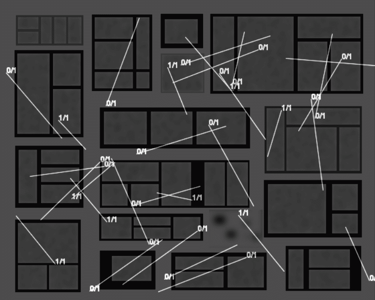
The baseline model uses a Boolean value for whether enough signal power is present to form a connection (Figure 5). A link budget is performed, given transmitter power, gains and losses, receiver gains, losses and sensitivity, and the calculated path loss, above. If the link budget is greater than 0 dB, then a connection is feasible.

We compared this baseline value against estimations made by two conventional models, and the RPEA model. The accuracy of a model refers to the proportion of results from the model that match the baseline value. That is, the proportion of times a model accurately predicts signal feasibility.

The first of the two conventional models used is the Friis’ free space path loss model [12]. Given the distance between communicating nodes, loss can be estimated as [19]:

L_AB [dB] ≈ 32.44 + 20logf [MHz] + 20logd [km]

where L_AB is the path loss between nodes A and B, f represents the frequency of the signal, assumed to be 2.4 GHz, and d is the distance between the two peers.

This models path loss given a line-of-sight communication path. As a built-up environment is being simulated for this comparison, this is not expected to yield generally accurate results.

For modelling the attenuation of radio signals by objects in the environment, a lognormal model is frequently used [20].

This includes a mean path loss component, as well as a zero-mean Gaussian distributed random variable, representing random shadowing effects due to movement of transmitter or receiver relative to attenuating objects. The second conventional model used for comparison is the lognormal model:

where L_AB is the path loss between nodes A and B, PL(d₀) represents the path loss at a pre-defined reference distance d₀, n is the path loss exponent, representing the amount of environmental clutter, and X_σ is a zero-mean Gaussian distributed random variable representing shadowing, with standard deviation σ.

The path loss exponent n characterises the environment. A path loss exponent of 2 corresponds to free space; a value of 2–3 generally corresponds to a semi-urban environment, and a value of 4–6 corresponds to more built-up environments [20]. For the purposes of comparison, a number of path loss exponent values were chosen during simulation.

Unlike conventional parametric models, the RPEA model makes use of a database that represents the radio propagation geometry of the surrounding environment. The fidelity of the RPEA database refers to how closely it resembles the radio propagation geometry of the environment. To profile the accuracy of the RPEA model given database fidelity, several pre-generated RPEA databases were used, with varying levels of fidelity. RPEA databases are derived from the baseline model’s attenuation map, and degraded fidelity is represented by a Gaussian blur, which approximates the effect of interpolation, present when little empirical information has been obtained. See the section below entitled ‘RPEA Model Sensitivity to Fidelity’ for further discussion.

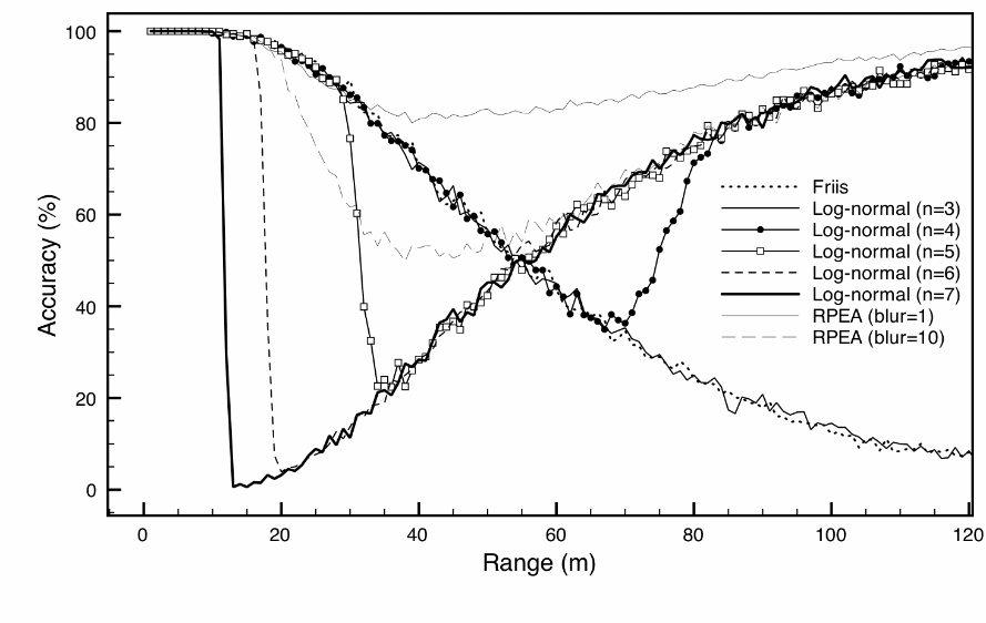
The results of simulation comparing the two conventional models with the RPEA model are depicted in Figure 6. Shown is the average prediction accuracy for each model and model variations, for peers communicating at a variety of ranges, i.e. distances between peers.

It can be seen that for small distances, accuracy is relatively high in all cases, as shadowing by dense objects has very little effect over such short distances, and prediction is trivial. Similarly, accuracy is quite high at the far distance, as the free space path loss components of each model dominate over shadowing effects, and can be easily calculated when distance is known.

Note that this also applies to the Friis free space model, and the lognormal model with n set to 3. Here, the predicted signal ranges are much greater than the simulated ranges, and thus do not converge with the simulated predictions for ranges less than several hundred metres.

Between these extremes in range, where accuracy is relatively high, accuracy drops off dramatically for all conventional models, as shadowing by objects in the environment has a significant effect on received signal power.

At these distances that are of the scale of the topographical features in the environment, no lumped attenuation parameter based on an average can accurately represent the attenuation upon a signal travelling through an inhomogeneous environment.

It is at these distances in particular where the RPEA model performs better than the conventional models.

Two mirrored curves are expressed in the results, which correspond to the distribution of present connections, and the distribution of absent connections. For the Friis free space model, corresponding to an empty environment with zero loss, the results conform to the curve representing the distribution of present connections. The accuracy of this model decreases with range, becoming rapidly less accurate as communicating pairs become more likely to be separated by attenuating objects.

This effect is reversed for the lognormal model with a path loss exponent n value greater than 3, modelling a more cluttered environment. Over larger distances, attenuation is more likely to have occurred by objects in the environment, thereby blocking the signal, in accordance with the estimate represented by the path loss exponent. However, at shorter distances, differences between the real world and the environment modelled by the path loss exponent become more apparent, as it is more likely that a communicating pair is separated by open space.

It is apparent from the results displayed in Figure 6 that the conventional model that best represents the simulated environment is the lognormal model with a path loss exponent of 4. This model yields accuracy of the order of 40% at distances of the scale of topographical features in the environment. This accuracy is surpassed by the RPEA model, even with degraded fidelity.

This result reveals that when the RF propagation environment details are not known, it is impossible to predict signal behaviour for communication links that span distances similar to the scale of the objects in the environment. Thus, using a conventional modelling process for the environment, such as those described above, does not yield accurate results for an inhomogeneous environment.

RPEA model sensitivity to fidelity

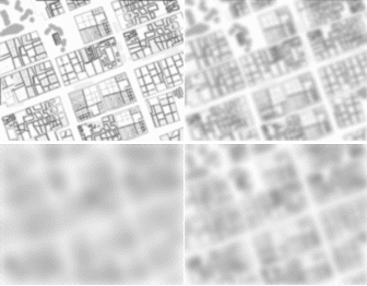
Figure 7 depicts the estimation accuracy of the RPEA model, given a knowledge map, and fidelity represented by a Gaussian blur.

A blur approximates the lack of sharpness caused by incomplete information in the model. This represents uniformly distributed information, resulting in a smooth image. A real-world model is more likely to have local regions of high information content, corresponding to a high node density of more populated regions of the surrounding environment. Future research will involve producing a large number of incomplete models, generated by an actual RPEA learning algorithm. For the purposes of this simulation, however, a Gaussian blur represents a tractable and quantifiable technique to represent restricted model fidelity.

The accuracy represented in Figure 7 is determined by the lowest accuracy given a number of simulation runs at various ranges between communicating nodes.

It can be seen that the best-case accuracy, of the order of 40%, using the conventional modelling methods described above, is surpassed by the RPEA model with degraded fidelity of 20m, approximately. This corresponding level of detail is very low, with no details apparent.

The RPEA result is demonstrably superior, despite impairments introduced by limiting the fidelity of the model database. The superiority of the RPEA model over the conventional model is highly insensitive to uniform degradation of the RPEA model database, as represented by a Gaussian blur.

Thus, we have shown that the RPEA model achieves better propagation loss prediction accuracy than a conventional parametric propagation loss model. In fact, the RPEA model performs better than a conventional model even with very low database fidelity, which suggests that even when little information about the local radio propagation geometry has been obtained, the RPEA model may still be superior to the conventional model.

Conclusion

Movement of nodes within an ad hoc network causes the network topology and parameters to be highly dynamic. Large objects in the environment exert a significant influence on RF signals, attenuating, diffracting, scattering and refracting signals to limit received power levels, and cause constructive and destructive interference. This impairs the network's connectivity and decreases link quality. By learning about the RF propagation environment, knowledge of the radio propagation geometry of the environment can be utilised in optimising network operation.

We showed through simulation that the model offered by RF Propagation Environment Awareness yields significantly more accurate estimation of signal behaviour than conventional methods, using parametric propagation models that do not incorporate local topographic features. We have also shown that high fidelity in the RPEA propagation model is not required to yield improvement over conventional methods, making feasible the presented approach.

Future work involves further developing appropriate learning algorithms and profiling their performance, given various effects such as location error, signal level measurement errors, multipath, and the modelling of reflection, diffraction and refraction effects.

Additional avenues for future research involve development of network management algorithms to exploit RPEA, including smart antenna control and route establishment and management, movement prediction algorithms to accurately predict future positions given past movement history, and database distribution to facilitate sharing of RPEA model information. Future research could also focus on the time-dependent nature of RF propagation, including RF interference from other equipment during different times of day, and weather effects.

Acknowledgments

Michael Tyson is supported by an Australian Postgraduate Award and a Victorian Government ICT Postgraduate Research Scholarship.

References

Authors

Michael Tyson, BCompSc graduated in 2005 with a Bachelor of Computer Science, First Class Honours, from Monash University’s Faculty of Information Technology, Melbourne, Australia, where he is currently undertaking a PhD. Michael's research interests include intelligent adaptive ad-hoc routing, radio propagation environment modelling, mobile station movement tracking and prediction, differential GPS over IP, power consumption optimisation and fairness in mobile ad-hoc networks, and ad-hoc network security. E-mail: mike@tyson.id.au.

Dr Carlo Kopp, IEEE, SMAIAA, PEng graduated from the University of WA in Electrical Engineering with First Class Honours, in 1984. After more than a decade in industry engineering positions he completed an MSc in 1996, and a PhD in 1999, the latter dealing with long range microwave datalinking via airborne radar phased arrays, and airborne ad hoc digital networks. He is currently at the Monash University Faculty of IT, with research interests in networking, security and information warfare. His other research interests include military technology and modern strategy. E-mail: carlo@infotech.monash.edu.au.

Ronald Pose completed his B.Sc.(hons) degree and his Ph.D. at Monash University, Melbourne, Australia. His Ph.D. involved the design and implementation of a novel capability-based operating system kernel. He joined the faculty of Monash University in 1988, where he has supervised a number of research students with whom he has worked on a wide variety of research projects including neural networks, genetic algorithm function optimization, network routing, low latency virtual reality address recalculation pipeline display system, and self-reconfigurable computer systems. Dr Pose's current research interests include virtual reality and telerobotics technology, computer architecture, parallel and distributed computer systems architecture, secure operating systems, reconfigurable computer systems architecture, multiprocessor interconnection networks, wireless ad hoc networks and spread-spectrum microwave communication technology, computer system security. E-mail: rd@infotech.monash.edu.au.

References

[1] C. Kopp, “Ad Hoc Networking,” Systems, pp. 33–40, July 1999.
[2] C E. Perkins and E.M. Royer, “Ad-hoc On-Demand Distance Vector Routing.” Proceedings of 2nd IEEE Workshop on Mobile Computing Systems and Applications, Feb. 1999.
[3] D. B. Johnson and D. A. Maltz, “Dynamic Source Routing in Ad Hoc Wireless Networks”, Mobile Computing, Imielinski and Korth, eds., Vol. 353, Kluwer Academic Publishers, 1996.
[4] S. Corson and J. Macker, Mobile Ad hoc Networking (MANET): Routing Protocol Performance Issues and Evaluation Considerations, RFC2501, January 1999.
[5] Y.-B. Ko and N.H. Vaidya, “Location-Aided Routing (LAR) in Mobile Ad Hoc Networks”, Wireless Networks, Vol. 6, pp. 307–321, September 2000.
[6] X. Lin and I. Stojmenovic, “Geographic Distance Routing in Ad Hoc Wireless Networks”, IEEE Journal on Selected Areas in Communication, 1998.
[7] W.-H. Liao, J.-P. Sheu, and Y.-C. Tseng, “GRID: A Fully Location- Aware Routing Protocol for Mobile Ad Hoc Networks”, Telecommunication Systems, Vol. 18, pp. 37–60, September 2001.
[8] Z.W. Cong, “Hybrid TDOA/AOA Mobile User Location for Wide-band CDMA Cellular Systems”, IEEE Transactions on Wireless Networks, Vol. 1, pp. 439–447, July 2002.
[9] N. Thomas, D. Cruickshank, and D. Laurenson, “Performance of a TDOA-AOA Hybrid Mobile Location System,” IEEE Conference Publications, vol. 2001, no. CP477, pp. 216–220, 2001.
[10] U.S. Air Force, “NAVSTAR GPS Space Segment/Navigation User Interfaces”, Interface Specification IS-GPS-200D, U.S. Air Force, March 2006.
[11] B.W. Parkinson and J.J. Spilker, “Global Positioning System: Theory and Applications”, American Institute of Aeronautics and Astronautics, 1996.
[12] J.S. Seybold, Introduction to RF Propagation, Wiley, 2005.
[13] H.J. Scudder, “Introduction to Computer Aided Tomography”, Proceedings of the IEEE, vol. 66, pp. 628–637, June 1978.
[14] A.C. Kak and M. Slaney, Principles of Computerized Tomographic Imaging, IEEE Press, 1998.
[15] A.G. Ramm and A.I. Katsevich, The Radon Transform and Local Tomography, CRC Press, 1996.
[16] J. Claerbout, Image Estimation By Example: Geophysical Soundings Image Construction, Stanford Exploration Project, 2 2006.
[17] M. Tyson and C. Kopp, “The Lightweight Global Navigation Satellite System (GNSS) Support Protocol (LGSP)” draft-tyson-lgsp-01, December 2007.
[18] SkyTel, Assisted GPS, Whitepaper, 5 2004.
[19] J.D. Parsons, The Mobile Radio Propagation Channel, Wiley & Sons Ltd., 2000.
[20] T. Rappaport, Wireless Communications Principles and Practice, Prentice Hall, 2001.