A Complex Mathematical Model For Computation Of The Dynamic Launch Zone For Air-To-Air Homing Missiles

Nomenclature

$\alpha$ - Angle of attack (AOA) (tangent definitions [8]);

$\beta$ - Sideslip angle (tangent definitions [8]);

${\gamma }_T$ - Target climb angle;

${\delta }_m$ - Canard deflection in pitch;

${\delta }_l$ - Canard deflection in roll;

${\delta }_n$ - Canard deflection in yaw [11];

${\theta }_M$ - LOS inclination angle [5];

$\theta$ - Inclination angle;

$\vartheta$ - Gimbal angle;

${\mu }_M$ - Aspect angle of missile;

${\mu }_T$ - Aspect angle of target;

$\rho$ - Air density [11];

$\phi$ - Bank angle [10];

${\chi }_T$ - Target track angle [5];

${\psi }_M$ - LOS azimuth angle;

$\psi$ - Azimuth angle;

${\omega }_M$ - Angular velocity of missile velocity vector;

${\omega }_T$ - Angular velocity of target velocity vector;

${\omega }_y,{\omega }_z$ - LOS angular velocity components in the guidance frame;

$\Omega$ - Missile angular velocity vector;

$a_M$ - Missile acceleration;

$a_x,a_y,a_z$ - Missile acceleration components in the guidance frame;

$a_T$ - Target acceleration;

$a_{\text{xT}},a_{\text{yT}},a_{\text{zT}}$ - Target acceleration components in the guidance frame;

$A,B,C$ - Missile inertia moments [11];

$C_l;C_m;C_n$ - Missile aerodynamic couples coefficients;

$C_x;C_y;C_z$ - Missile aerodynamic forces coefficients;

$g$ - Gravity acceleration;

$H$ - Altitude;

$l$ - Missile reference length;

$M$ - Missile;

$m$ - Missile mass;

$M_A$ - Airplane Combat Mach number;

$M_T$ - Target Mach number;

$M-T$ - Line of sight (LOS) - Connective line between missile and target;

$n_M$ - Load factor of missile;

$n_T$ - Load factor of target;

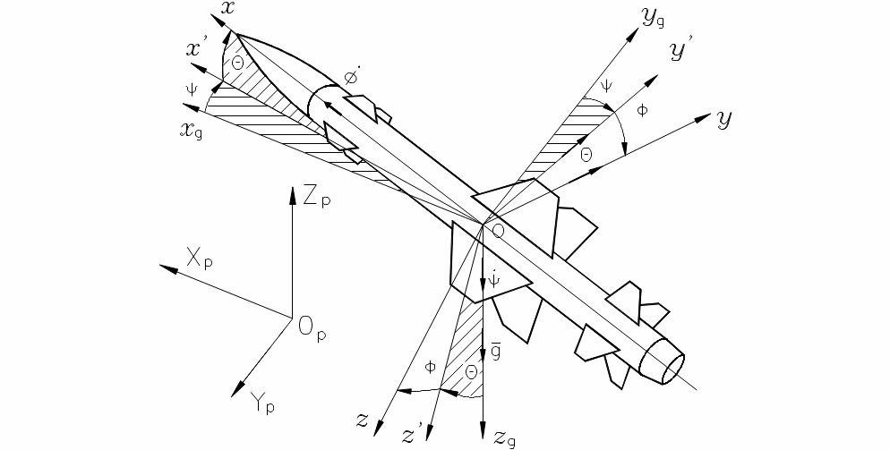
$\text{Oxyz}$ – Missile body frame (mobile frame);

${\text{OX}}_T{Y}_T{Z}_T$ - Guidance frame [5];

${\text{OX}}_p{Y}_p{Z}_p$ - Normal Earth-fixed frame [3];

$p,q,r$ - Angular velocity components along the missile body frame axis [11];

$\tilde{q}=\rho \frac{V^2}{2}$ - Dynamic pressure;

$R$ - Distance between missile and target (range);

$S$ - Missile reference area;

$T$ - Target;

$T$ - Missile thrust;

$u,v,w$ - Velocity components in the missile body frame [10];

$V$ - Missile velocity vector [10];

$V_A$ - Airplane Combat (A/C) velocity;

$V_T$ - Target velocity;

$x_p{y}_p{z}_p$ - Missile coordinates in Earth-fixed frame;

$x_{\text{Tp}}{y}_{\text{Tp}}{z}_{\text{Tp}}$ - Target coordinates in Earth-fixed frame [5];

$x_{\text{cm}}$ - Missile mass center position relative to nose [5].

Introduction

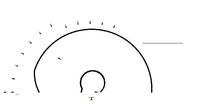
One of the main tasks of the Aircraft Combat (A/C) System designer is to define the performance of the armament that will allow the pilots to use their own system at full capability. One of the armament performance aspects is linked to the Dynamic Launch Zone (DLZ) of missiles, particularly for homing air-to-air missiles. The issue is important both technically and commercially because customers are reluctant to buy such a system without knowing its performance, which means that the designer will have to consider providing such technical information. Reference [7] provides some ideas and results, but it doesn’t reveal the mathematical model behind them. Technically speaking, the DLZ problem consists in obtaining, for any tactical combat situation, the launch zone limits (Figure 1).

Problem statement

As we can see in Figure 1 the DLZ problem can be split in two different sub–problems: outside limit computation and inside limit computation. The outside limit is given by the maximum distance ($R_{\text{max}}$) at which the missile can be successfully launched against the target. The inside limit is given by the minimum distance ($R_{\text{min}}$) from which the missile can be successfully launched against the target. The tactical situations are defined by four parameters: altitude of the A/C and target, Mach number of the A/C at the launch moment ($M_A$), Mach number of the target ($M_T$), and the load factor of the target ($n_T$). These parameters define the initial conditions of the DLZ problem.

General assumptions

The following mathematical model is based on the following general assumptions:

a) The initial gimbal angle is zero.

b) The maximum distance to the target, provided by radar is not considered, due to its strongly variable nature, depending on weather conditions.

c) Launch time delay is zero.

d) The altitudes of the A/C and the target are equal.

e) The target flights at constant velocity and constant maneuver during the interception process.

f) The target is not heading towards the A/C (it is not conducting a suicide maneuver).

In non-maneuver target case, the DLZ is symmetrical, so that the two halves are computed in the same way. Assumption (f) is possible because, in maneuver target cases, we are interested only in the half zone related to possible target maneuver.

General restrictions

The calculus was performed in the particular case of the following numeric example:

a) Maximum LOS rate of turn 30 [deg/s];

b) Maximum gimbal angle 55 [deg]

c) Safe time of the fuze (TOF) 1.45 [s]

d) Maximum canard deflection 20[deg]

e) Maximum time of guided flight 25 [s]

f) Maximum load factor for missile 50

g) Closure rate, correlated to the Doppler fuze 98 [m/s]

Mathematical model and input data

The DLZ–complex model consists in the nonlinear equations of the missile motion (kinematical and dynamic equations), the equations of target in the fixed frame, the LOS velocity equations in the guidance frame, the equations of the seeker in the guidance frame (the command relations), the actuator equations and the general restrictions.

The complex model assumes that the following input data are known: the aerodynamic characteristics of the missile; the thrust diagram; mass characteristics (mass, inertia momentums and mass center), and the guidance characteristics.

The nonlinear equations of motion

The nonlinear equations in the general form can be found in [3,5−7]. Briefly, they are described in the following sections.

a) The kinematical equations

Velocity equations link velocity components expressed in missile frame coordinates, to velocity components expressed in fixed frame coordinates.

where:

$B_p=\left[\text{cos}\psi \text{cos}\theta \begin{array}{c}-\text{s}\text{i}\text{n}\psi \text{c}\text{o}\text{s}\phi +\\ +\text{c}\text{o}\text{s}\psi \text{s}\text{i}\text{n}\theta \text{s}\text{i}\text{n}\phi & \text{s}\text{i}\text{n}\psi \text{s}\text{i}\text{n}\phi +\\ +\text{c}\text{o}\text{s}\psi \text{s}\text{i}\text{n}\theta \text{c}\text{o}\text{s}\phi \\ -\text{sin}\psi \text{cos}\theta & -\text{c}\text{o}\text{s}\psi \text{c}\text{o}\text{s}\phi -\\ -\text{s}\text{i}\text{n}\psi \text{s}\text{i}\text{n}\theta \text{s}\text{i}\text{n}\phi & \text{c}\text{o}\text{s}\psi \text{s}\text{i}\text{n}\phi -\\ -\text{s}\text{i}\text{n}\psi \text{s}\text{i}\text{n}\theta \text{c}\text{o}\text{s}\phi \\ \text{sin}\theta & -\text{cos}\theta \text{sin}\theta & -\text{cos}\theta \text{cos}\phi \end{array}\right]$

Angular velocity equations (Euler kinematical equations) link the components of angular velocity $\Omega (p,q,r)$ expressed in missile frame to the attitude angle ($\psi$,$\theta$,$\phi$) derivatives.

where:

b) The dynamic equations in the missile frame contain [5]:

Force equations.

where: $A_p=B_p^T$, and $F_0=\tilde{q}S$ is the aerodynamic reference force.

Moment equations (Euler’s dynamic equations):

with: $H_0=F_{0}l$ aerodynamic reference moment and

the inertial moment inverse matrix. The inertial moments are given by:

For practical computations, we used the following quantitative data:

- Reference length: $l=2\text{.}\text{73}m$;

- Reference area: $S=0\text{.}\text{0194}{m}^2$;

- For active phase (the missile start):

$m_i=\text{90}\text{kg}$; $x_{\text{cmi}}=1\text{.}\text{49}m$;

$A_i=0\text{.}\text{403}{\text{kgm}}^2$; $B_i=C_i=\text{57}\text{.}\text{34}{\text{kgm}}^2$.

- For passive phase (after burn out):

$m_f=\text{67}\text{kg}$; $x_{\text{cmf}}=1\text{.}\text{39}4\text{m}$;

$A_f=0\text{.}\text{354}{\text{kgm}}^2$; $B_f=C_f=\text{47}\text{.}\text{38}{\text{kgm}}^2$.

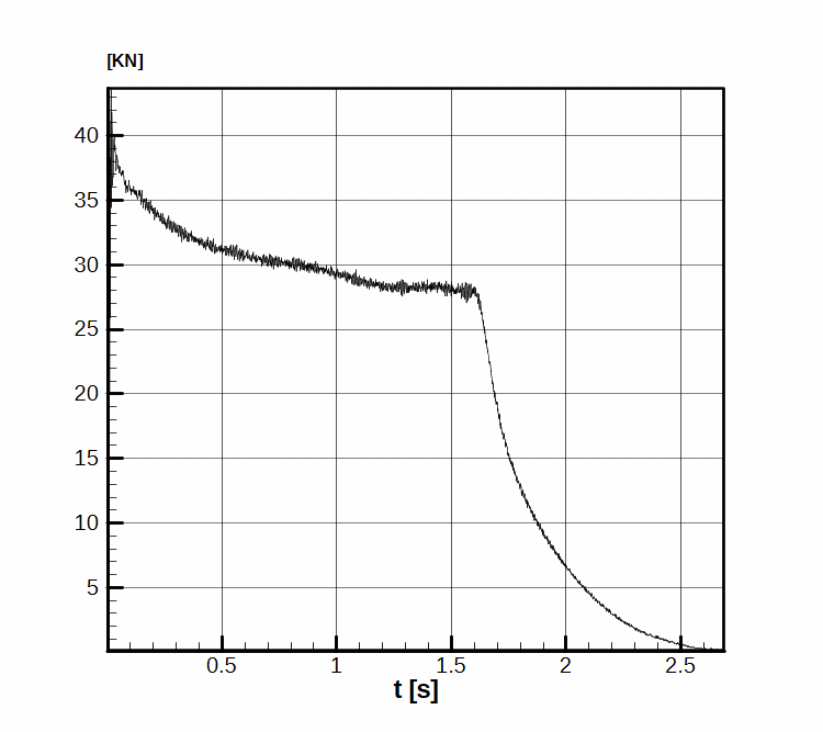
The missile thrust force diagram used in our analysis is shown in Figure 3. This diagram was obtained by averaging two experimental thrust data ranges obtained in a Romanian test facility [13].

For the aerodynamic coefficients calculus we used the method indicated in [1] and [8], based on polynomial series expanding:

$C_x=a_1+a_2({\alpha }^2+{\beta }^2)+a_3({\alpha }^4+{\beta }^4)+a_4{\alpha }^2{\beta }^2+a_6({\delta }_m^2+{\delta }_n^2)+a_7{\delta }_l^2+\text{.}\text{.}\text{.}$$C_y=-b_1\beta -b_2{\beta }^3-b_3{\alpha }^2\beta -b_4\widehat{r}-b_5{\delta }_n-b_6({\alpha }^2+{\beta }^2){\delta }_n-b_9\widehat{\beta }+\text{.}\text{.}\text{.}$$C_z=b_1\alpha +b_2{\alpha }^3+b_3{\beta }^2\alpha +b_4\widehat{q}+b_5{\delta }_m+b_6({\beta }^2+{\alpha }^2){\delta }_m+b_9\widehat{\alpha }+\text{.}\text{.}\text{.}$$C_l=c_2({\alpha }^2+{\beta }^2)\text{αβ}+c_3\widehat{p}+c_5(\alpha \widehat{q}-\beta \widehat{r})+c_6{\delta }_l+c_7({\alpha }^2+{\beta }^2){\delta }_l+\text{.}\text{.}\text{.}$$C_m=d_1\alpha +d_2{\alpha }^3+d_3{\text{αβ}}^2+d_4\widehat{q}+d_5{\delta }_m+d_6({\alpha }^2+{\beta }^2){\delta }_m+d_9\widehat{\alpha }+\text{.}\text{.}\text{.}$$C_n=d_1\beta +d_2{\beta }^3+d_3{\alpha }^2\beta +d_4\widehat{r}+d_5{\delta }_n+d_6({\alpha }^2+{\beta }^2){\delta }_n+d_9\widehat{\beta }+\text{.}\text{.}\text{.}$ (7)

where $\alpha =-\text{arctan}/$; $\beta =\text{arctan}/$, as stated in [8].

The notations used for the non-dimensional angular velocities:

and for the non dimensional and non stationary attack and sideslip angles:

where $V$ is magnitude of velocity vector.

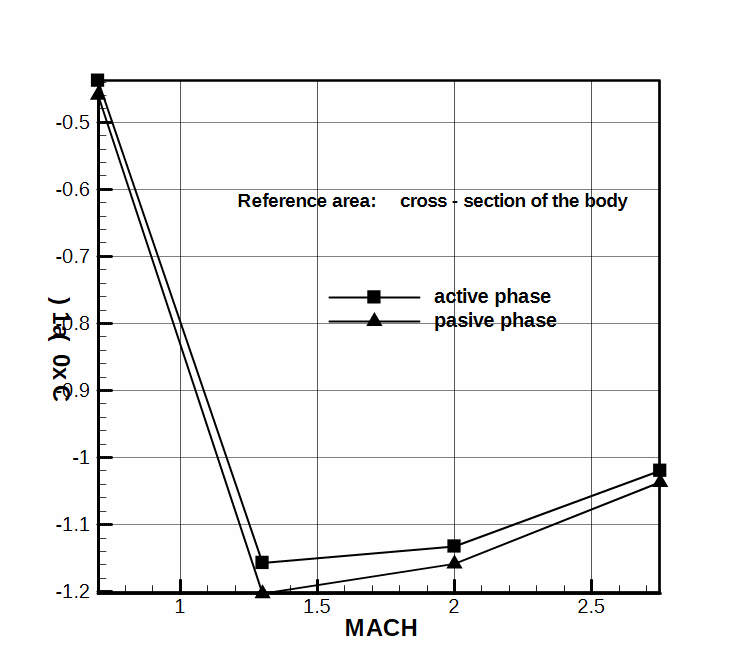
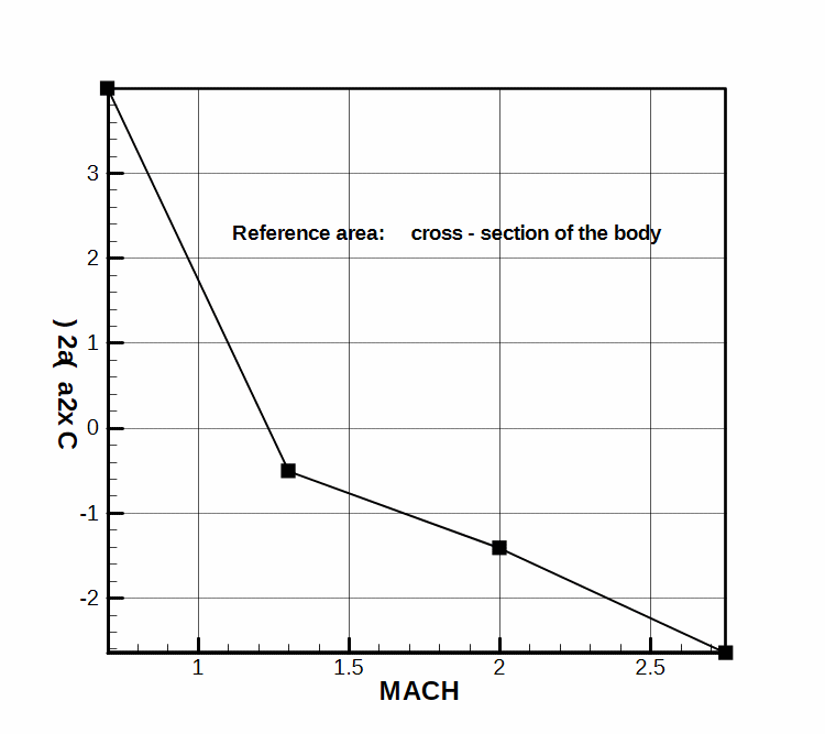
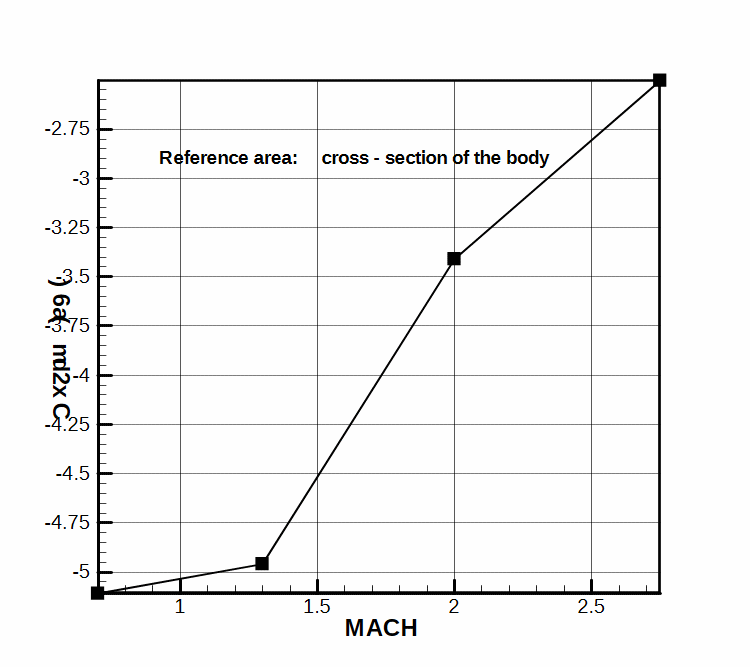
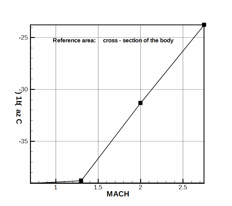
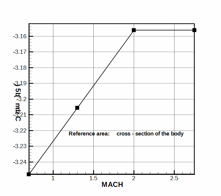
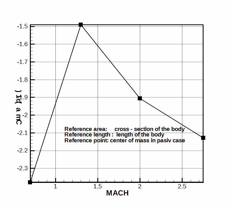
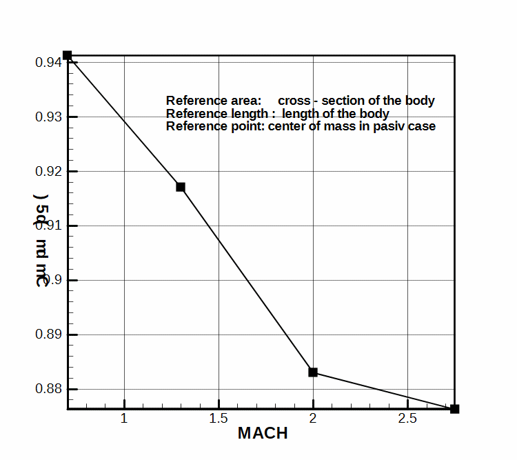
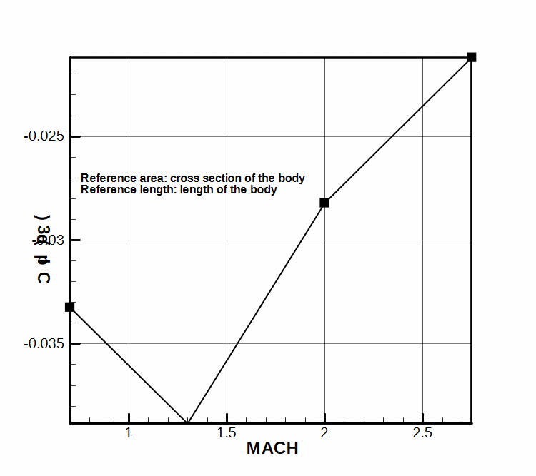
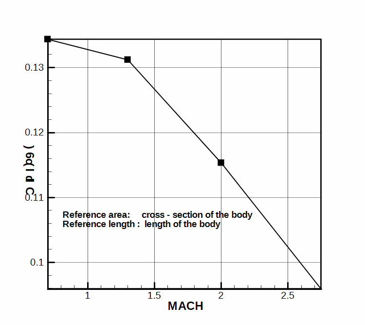
The coefficients $a_1,a_2,\text{.}\text{.}\text{.}{b}_1,b_2\text{.}\text{.}\text{.}{d}_1,d_2$ from Equations (7) are presented in the next figures. In Figures 4 to 12 we show the experimental diagrams of the main coefficients derivatives variation versus Mach number [12].

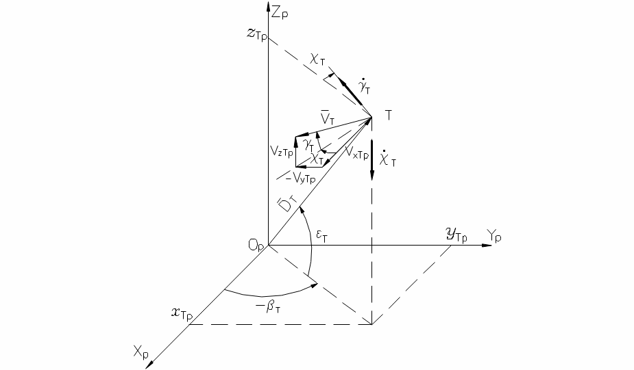
c) Target kinematical equations in the Earth frame [4,9]:

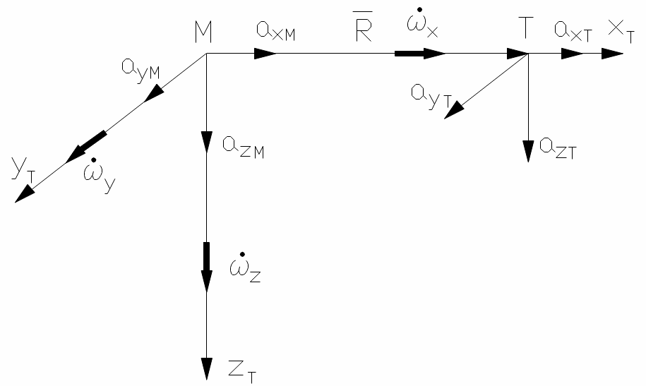
d) LOS velocity equations in the guidance frame [2,4−6]:

where:${\tilde{a}}_{\text{zT}}=a_{\text{zT}}-a_z$ and ${\tilde{a}}_{\text{yT}}=a_{\text{yT}}-a_y$ are relative accelerations along the guidance frame.

e) Seeker equations in the guidance frame [2,5]:

where:$u_y$; $u_z$ -guidance signals, $k_u^{\omega }=\text{40}\cdot (-\dot{R})/g$−seeker’s gain [s]; ${\tau }_c=0\text{.}\text{01}s$−seeker’s time constant, ${\omega }_y,{\omega }_z$−LOS angular velocity components in the guidance frame, obtained from Equations (11).

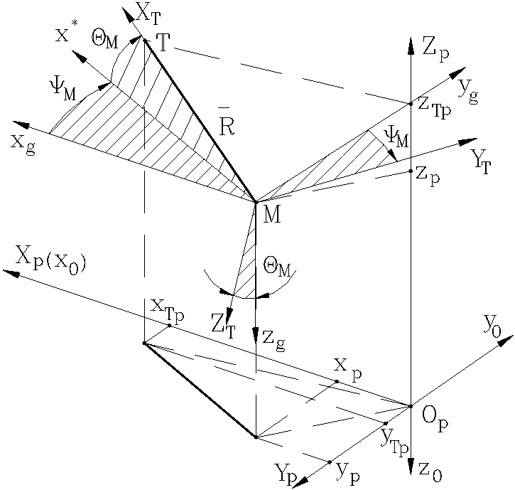
f) Command relations (autopilot relations) from guidance frame to missile mobile frame:

$u=[u_l{u}_m& u_n{]}^T$ are the command signals.

The scalar form for the signals:

where the elements of the transformation from the guidance frame to the missile body mobile frame are:

$a_{\mathrm{2,2}}=\text{sin}\phi \text{sin}\theta \text{sin}(\psi -{\psi }_M)+\text{cos}\phi \text{cos}(\psi -{\psi }_M);\begin{array}{c}{a}_{\mathrm{2,3}}=\text{s}\text{i}\text{n}\phi \text{s}\text{i}\text{n}\theta \text{s}\text{i}\text{n}{\theta }_M\text{c}\text{o}\text{s}(\psi -{\psi }_M)-\text{c}\text{o}\text{s}\phi \text{s}\text{i}\text{n}{\theta }_M\text{s}\text{i}\text{n}(\psi -{\psi }_M)+\\ +\text{s}\text{i}\text{n}\phi \text{c}\text{o}\text{s}\theta \text{c}\text{o}\text{s}{\theta }_M;\\ a_{\mathrm{3,2}}=\text{cos}\phi \text{sin}\theta \text{sin}(\psi -{\psi }_M)-\text{sin}\phi \text{cos}(\psi -{\psi }_M);\\ a_{\mathrm{3,3}}=\text{c}\text{o}\text{s}\phi \text{s}\text{i}\text{n}\theta \text{s}\text{i}\text{n}{\theta }_M\text{c}\text{o}\text{s}(\psi -{\psi }_M)+\text{s}\text{i}\text{n}\phi \text{s}\text{i}\text{n}{\theta }_M\text{s}\text{i}\text{n}(\psi -{\psi }_M)+\\ +\text{c}\text{o}\text{s}\phi \text{c}\text{o}\text{s}\theta \text{c}\text{o}\text{s}{\theta }_M;\end{array}$(14)

with the angles which define the guidance frame given by:

${\psi }_M=-\text{arctg}\frac{y_{\text{Tp}}-y_p}{x_{\text{Tp}}-x_p};{\theta }_M=\text{arctg}\frac{z_{\text{Tp}}-z_p}{\sqrt{{\left(x_{\text{Tp}}-x_p\right)}^2+{\left(y_{\text{Tp}}-y_p\right)}^2}}\text{.}$ (15)

The roll relative angle is:

where:${\phi }_D=\pi /4$;

The load factors from Equations (13) (number of “g’s”), are defined by:

The constant values for command relations are:

$k_u^{\Phi }=1\text{.}0$; $k_u^p=0\text{.}1$; $k_u^q=k_u^r=7\text{.}5$; $k_u^n=1\text{.}$

g) Actuator equations in the body mobile frame are:

${\dot{\delta }}_l=-\frac{{\delta }_l}{{\tau }_{\delta }}+\frac{k_{\delta }^u{u}_l}{{\tau }_{\delta }};{\dot{\delta }}_m=-\frac{{\delta }_m}{{\tau }_{\delta }}+\frac{k_{\delta }^u{u}_m}{{\tau }_{\delta }};& {\dot{\delta }}_n=-\frac{{\delta }_n}{{\tau }_{\delta }}+\frac{k_{\delta }^u{u}_n}{{\tau }_{\delta }}\text{.}$

(18)

where constant values were used for $k_{\delta }^u=0\text{.}\text{03}$ and ${\tau }_{\delta }=0\text{.}\text{001}\left[s\right]$

h) Calculus algorithm

To integrate the nonlinear equation system we used a multi-step method Adams’ predictor-corrector with variable step integration method [9,11]. The algorithm precision was estimated at 10^-7 for the absolute error and 10^-5 for the relative error.

Preliminary results

Firstly, we considered the case of the A/C and target in horizontal flight, with the command relation similar to (13), only that the terms:$u_l,u_m,u_n$ will contain the angular control of missile and flight altitude [5]. The horizontal trajectory of the missile obtained from computation follows a straight way, characterized by the velocity diagram in Figure 16 and the space diagram in Figure 17.

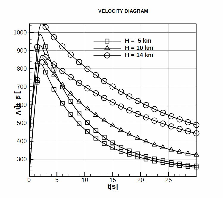
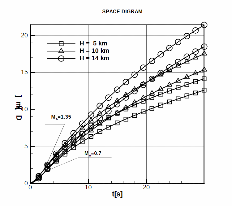
From these preliminary results, we could appreciate the maximum range of the missile for several initial conditions (different A/C velocity or altitude). The velocity and space variation for subsonic and supersonic A/C in case of launching at various altitudes (5 km, 10 km, 14 km) are show in the Figures 16 and 17.

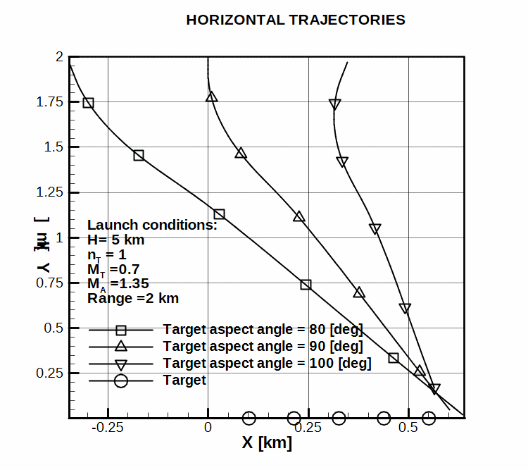
Using the “command relations” in (13) we analyzed two tactical cases. Firstly, we considered a maneuvering target $(n_T=1)$ at Mach number$M_T=0\text{.}7$, starting from origin at the same time with the missile with the initial conditions $M_A=1\text{.}\text{35}$ and $H=5\text{km}$. We considered the cases at the same initial range$R=2\text{km}$, given by different aspect angles of the target: ${\mu }_T=\text{80}°$; ${\mu }_T=\text{90}°$;.${\mu }_T=\text{100}°$.

From Figure 18 we can observe that for the first two cases, the missile hits the target, while for the initial aspect angle${\mu }_T=\text{100}°$, the missile misses the target.

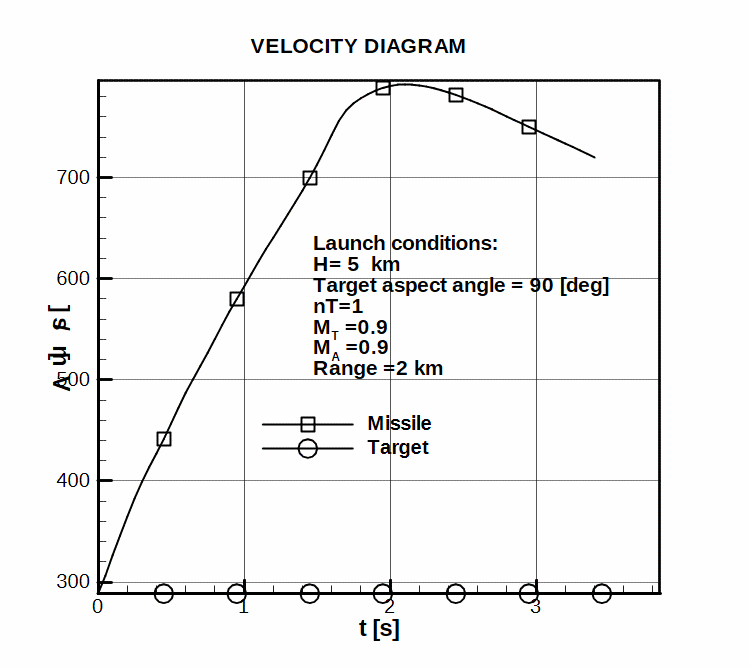
In Figure 19 we can see the missile and target velocities variation in time, for the first case.

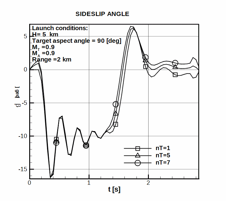
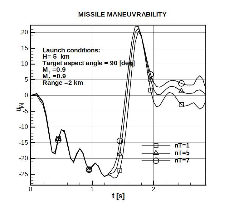
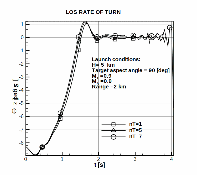
Secondly, we considered three cases (Figure 20), where the target and the A/C have the same Mach number $M_A=M_T=0\text{.}9$, the same altitude $H=5\text{km}$, the same initial target aspect angle ${\mu }_T=\text{90}°$ but different target load factors: $n_T=1$, $n_T=5$, $n_T=7$.

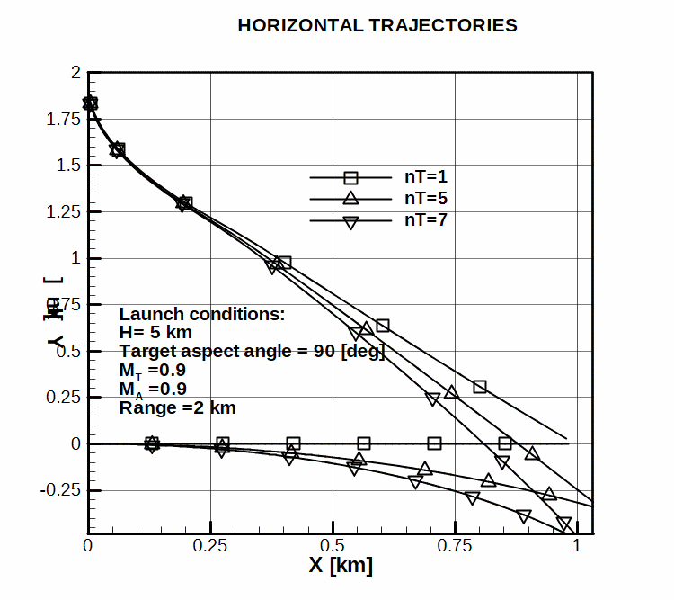
For each case, the missile hits the target, which means that the guidance parameters do not exceed the values previously indicated at “General restrictions” from Section 2.

In Figure 21 the canard yaw deflection can be seen and noticed that for any load factor, the maximum value 20[deg] isn’t exceeded.

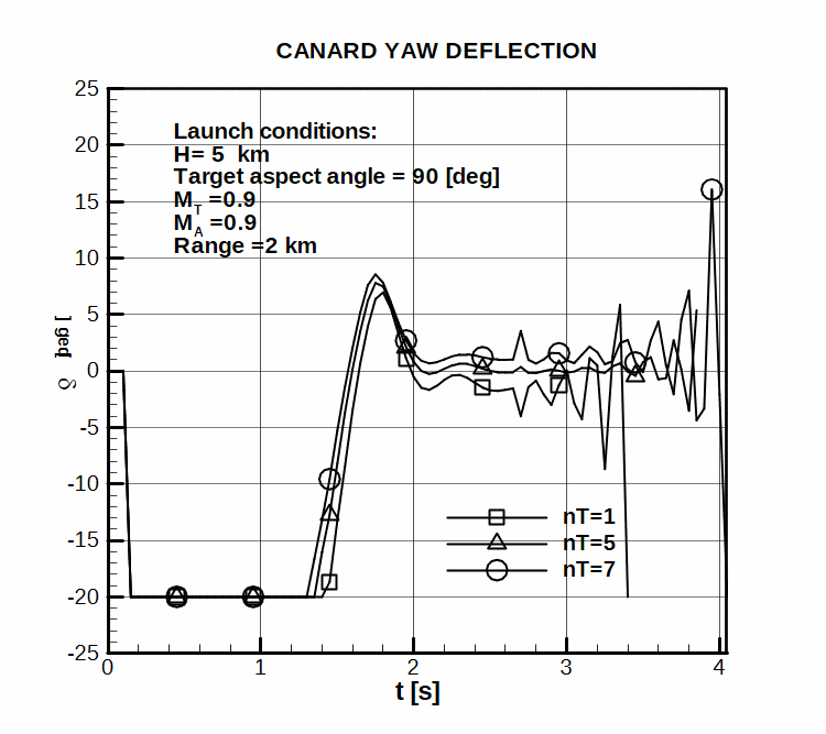
Figure 22 shows the sideslip angle during flight evolution, which remains between normal limits. This means that the aerodynamic characteristics described in relation (7) and presented in Figures 4 to 12, were correctly used.

The missile load factor for different target load factor can be seen in Figure 23. This diagram can be use to evaluate the missile load factor and compare it with the maximum allowed value.

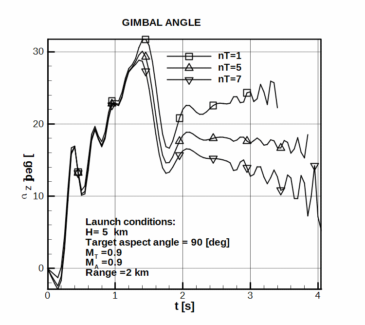
Finally, in Figure 24 and 25 we present the variation of the main guidance parameters: LOS rate of turn and gimbal angle, versus time. It can be observed that they do not exceed the maximum values previously indicated: maximum LOS rate to turn 30 [deg/sec] and maximum gimbal angle 55 [deg].

The mathematical model described above could be used for computation of the dynamic launch zone parameters.

Dynamic launch zone for air-to-air homing missile

To define the initial conditions, we considered the tactical situation when the interception is in the horizontal plane, which allowed outside and inside limits to be calculated in polar coordinates (range $R$ and aspect angle of target ${\mu }_T$). The initial parameters are defined depending on the above tactical situation:

$H=\text{constant}$ ;

$n_T=\text{constant}$;

$M_T=\text{constant}$;

$M_A=\text{constant}$.

For the aspect angle of the target ${\mu }_T$, we initiated an iterative cycle, with constant angle ($5°$) between $0°$ and $\text{180}°$, covering 37 cases. For each case we obtained the range for outside $R_{\text{max}}$ and inside $R_{\text{min}}$ limits. More explicit, we enclose one of the limits, say $R_{\text{max}}$, between two shooting trajectories, one of them hitting the target and another missing the target. We split the interval between the two ranges in two halves and chose the one of which enclosed $R_{\text{max}}$. When the interval obtained is small enough (1m) we considered that the solution was found. Then, we repeated the algorithm to find out $R_{\text{min}}$. After the solutions for both limits were obtained, we changed the aspect angle and repeated the algorithm. Time to obtain the solution for the 37 cases, to both limits, was 30 min.

A) launch envelopes for non-maneuvering target

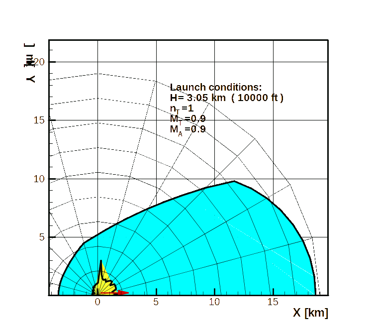
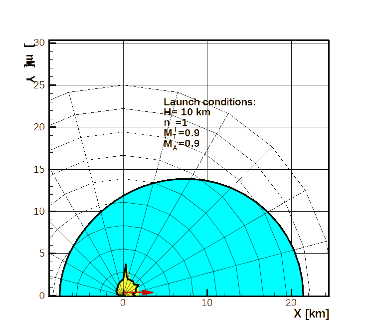
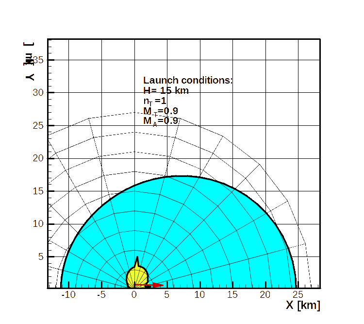
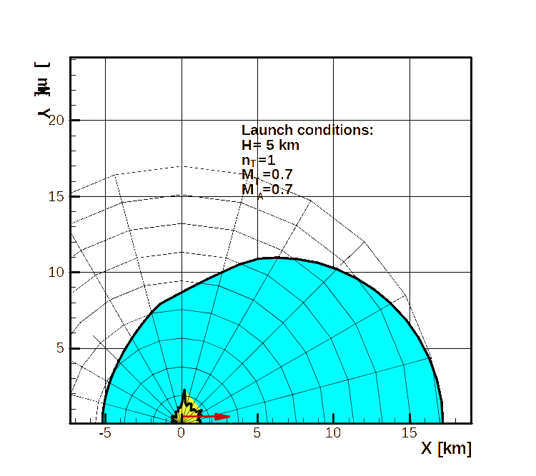
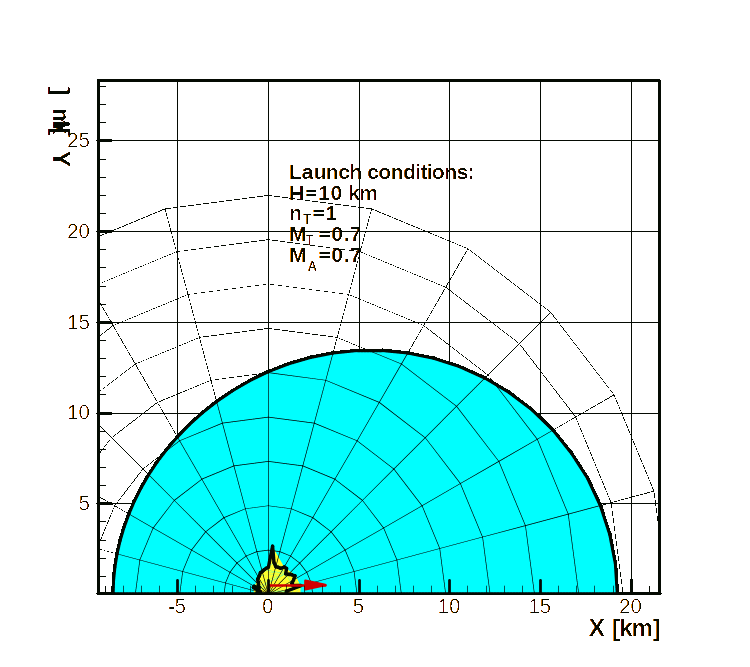
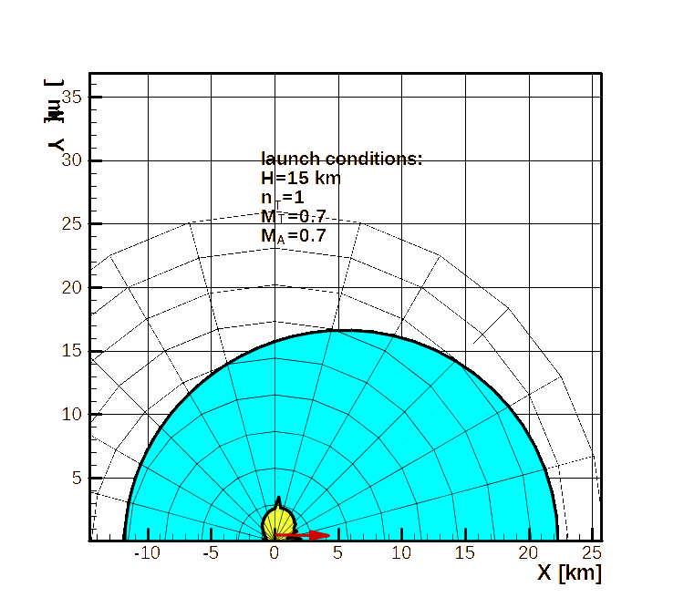
To analyze the DLZ obtained by the complex model presented above we considered six tactical situations, for subsonic and transonic A/C and target, and non maneuvering target. These cases are synthesized in Table 1.

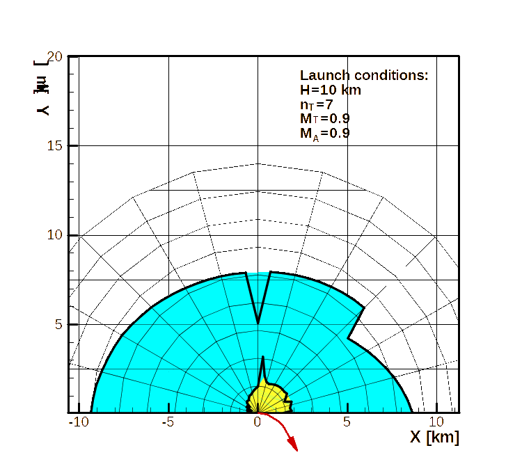
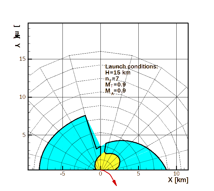
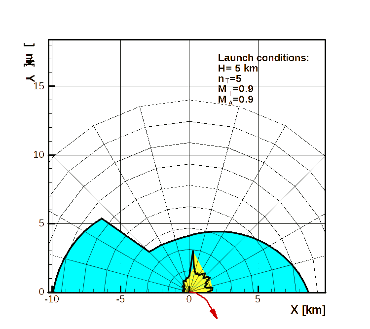
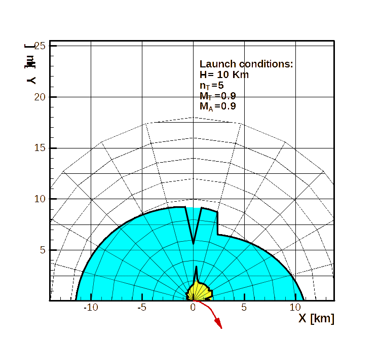
The results are shown in the Figures 26 to 31. In Figure 26 we can see the case of transonic A/C and target for low altitude. In Figure 27 we present the case of transonic A/C and target at medium altitude and in Figure 28 it is shown the case of transonic A/C and target at high altitude. In Figure 29 we present the subsonic A/C and target at low altitude, in Figure 30 subsonic A/C and target at medium altitude and finally in Figure 31 subsonic A/C and target at high altitude.

B) launching envelopes maneuvering target

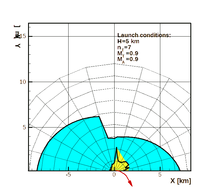
To complete the DLZ analysis with the complex model we considered six other tactical situations, for transonic A/C and target for high and medium maneuvering target. These six cases are synthesized in Table 2.

The results for these cases are shown in Figures 32 to 37. Thus, in Figure 32 we present the case of high maneuvering target for low altitude. In Figure 33 we present the case of high maneuvering target at medium altitude and in Figure 34 it is shown the case of high maneuvering target at high altitude. In Figure 35 we present the medium maneuvering target at low altitude, in Figure 36 the medium maneuvering target at medium altitude and finally in fig 37 the medium maneuvering target at high altitude.

Conclusions

Some relevant conclusions can be obtained by synthesis of the previous results—shown in Figures 38 to 41. In Figure 38 we present the outside limit for non- maneuvering target at different altitudes. As we presented in [5], for low altitude, the outside limit depends on restrictions such as: maximum time of guided flight, maxim gimbal angle or maximum LOS rate of turn, because the velocity decreases rapidly at low altitude. For high altitude, where the velocity decreases slowly, only one restriction is important: the maximum time of guided flight, necessary to define the outside limit. For this reason, the outside limit for altitude higher than 10 km is a circle, with the origin translated with distance covered by the target during the missile flight. If we compare this diagram with the space diagram in Figure 17 (space for the maximum time of guided flight), we observe a good match between the results, especially at high altitude can be obtained.

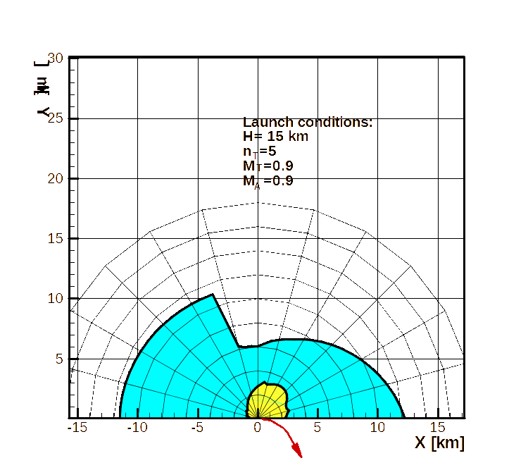
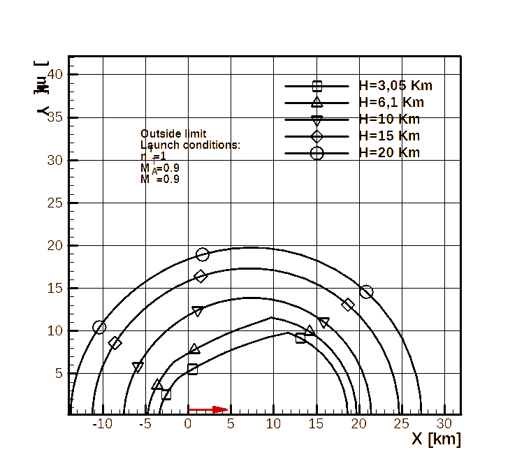
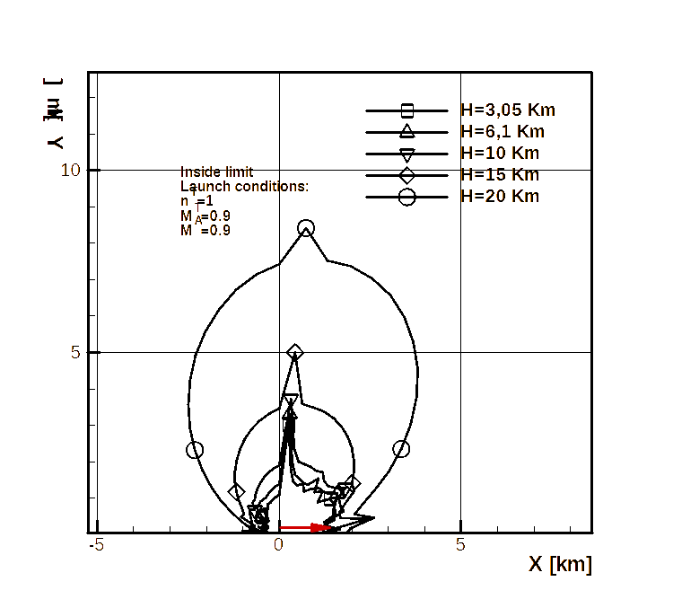
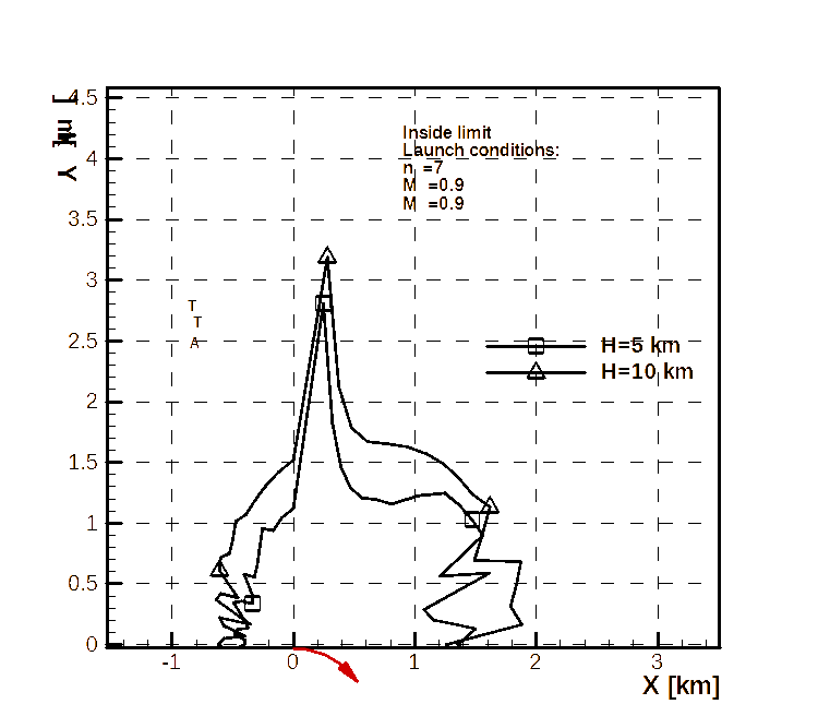
Figure 39 illustrates the inside limit for non- maneuvering target at different altitudes. This limit depends particularly on the maximum LOS rate of turn or maximum maneuver capacity of the missile. One can observe that this limit increases with altitude because the maneuver capacity of the missile decreases with altitude. As we presented in [5], safe time of the fuse (TOF) influences the inside limit only for target aspect angles around 0 deg or 180 deg.

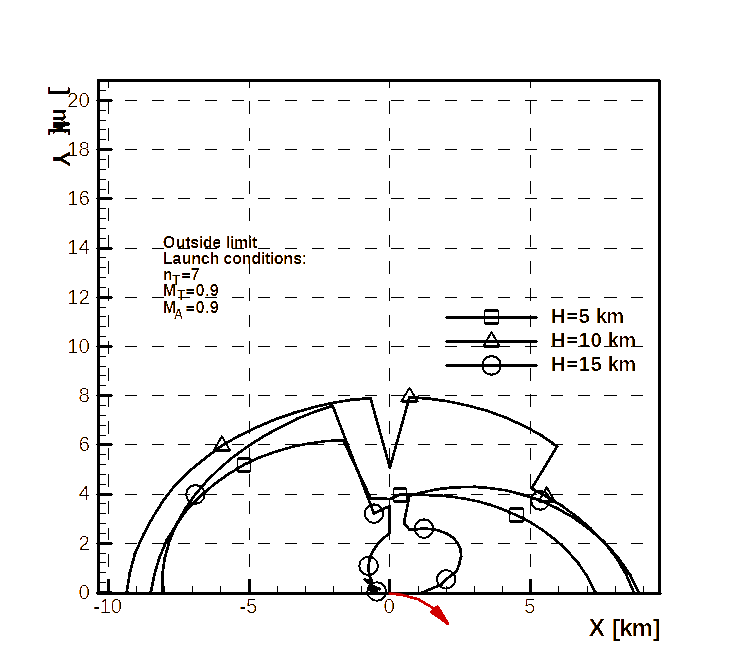
In Figure 40 we present the outside limit for high maneuvering targets at several altitudes. Similarly with a non-maneuvering target, the restrictions which influence the outside limit are the same but their weight is different. Additionally, the outside limit can be influenced by the maneuvering capacity of the missile. As can be seen in Figure 40, the outside limit has the tendency to grow with altitude, but a general trend is difficult to estimate.

In Figure 41 we present the inside limit for high- maneuvering target at several altitudes. As with non-maneuvering cases, this limit depends particularly on maximum LOS rate of turn, the maximum maneuver capacity of the missile and the TOF. It can be observed that this limit increases with altitude, while the maneuver capacity of the missile decreases.

Finally, we considered the accuracy of the model related to the real tactical situation. Obtaining experimental results regarding missile performances is a very expensive task, because it involves a large amount of resources for different tactical situations and also requires the destruction of many missiles and targets. For this reason, a more realistic and efficient approach could be developed only by a similar model as presented here, which can assist in the evaluation of the accuracy of the results by the accuracy of the input data and the complexity of the model itself. For this reason, the model presented uses only experimental data as input. The dynamic and kinematical equations used are expressed without approximations. The complex model presented is the best model that we could obtain with available experimental data, but it can be improved by using a more complete experimental data and a more precise model regarding the guidance system. However, this model is too slow to be used in real time, because one tactical case can be solved in approximately 1 min, which is too long for a real aerial fight situation. In this case, it is necessary to develop a simplified model, which may provide a less accurate, but still acceptable solution to be used for the weapon system software of an A/C computer.

References

Authors

Teodor-Viorel Chelaru completed his PhD studies in 1994. Since 1984 he has participated in a number of projects for guided and unguided missiles and UAV inside of the National Company for Military Technique. He is an Associate Professor at the POLITEHNICA University of Bucharest. His main research is focused on the dynamic flight and control of guided missiles.

Mircea Cernat completed his PhD in 1996. He is the deputy director for science at Military Equipment and Technology Agency, Bucharest. Since 1987 he has worked in positions linked to education and research, having the title of professor at Military Technical Academy in Bucharest. He has managed or contributed as a member in research teams in several projects regarding weapon systems technology. His research topics are focused on applied mathematics to weapon systems and structural mechanics. Phone: +40-21-423.14.83, e-mail: mcernat@acttm.ro, fax +40-21-423.10.30.

References

[1] СВЯТОДУХ,В.К., Динамика пространсвенново управляемых ракет, Издательство “Машиносроение” Москва, 1969.
[2] Belea, C., Lungu, R., Cismaru, C., Sisteme giroscopice şi aplicaţiile lor, Ed. Scrisul Românesc, Craiova, 1986.
[3] Boiffier, J.L., The Dynamics of Flight – The Equations, John Wiley & Sons , Chichester, New York, Weinheim, Brisbane, Singapore, Toronto , ISBN 0-471-94237-5, 1998.
[4] Carpantier,R., Guidance des avions et des missiles aerodynamiques. , Tom I,II,III, lit. ENSAE - 1989.
[5] Chelaru T.V., Dinamica Zborului–Racheta dirijată, Ediţia a-II-a revizuită şi adaugită ,Ed.Printech, Bucureşti, ISBN 973-718-013-5 , mai 2004.
[6] Chelaru T.V., Dinamica Zborului – Proiectarea avionului fără pilot , Ed. Printech, Bucureşti, ISBN 973-652-751-4, aprilie 2003.
[7] KaЗakoB,И.E., MИШakov,A.Ф., Aвиационные управляемые ракеты, Издание ВВИА „НЕ ЖУКОВСКОГО” ,1985.
[8] Niielsen J.N., Missile Aerodynamics, Mcgraw-Hill Book Company, Inc. New York, Toronto, London, 1960.
[9] Bakhvalov, N. Methodes Numeriques—Analyse, algebre, equations differentielles ordinaires Ed. Mir Moscou , 1976.
[10] ISO 1151 -1:1988; -2:1985-3:1989.
[11] SLATEC Common Mathematical Library, Ver 4.1, July 1993.
[12] Şelescu R, Costian L. Testare macheta in suflerie, Raport experimental INCAS , cod c-3020 / 2003.
[13] Sava, C, Matis, C, Testare motor rachetă, Raport experimental, SC Electromecanica Ploieşti SA, contr. 24/ 2003.