Complexity-Based Assessment In Crowd Confrontation Modelling

Introduction

Combat modelling and simulations are an integral part of military operational research. One of the greatest challenges for the analytical community is the evaluation of results. Measures of effectiveness (MOE) traditionally used to assess outcomes of combat modelling are mostly attrition-based. The attrition-based MOEs often provide only a limited battlefield picture, even in force-on-force scenarios, especially with respect to force manoeuvres. They usually focus on the end state, while ignoring the temporal and the spatial dynamics of the modelled combat [1]. Furthermore, the impact of incapacitating key targets such as command and control (C2) nodes is often ignored [2].

While reasonably well suited (despite the above-mentioned limitations) for typical force-on-force operations, these MOEs have a very limited applicability in modelling operations in which the preferred end state involves no casualties at all, such as peace support operations, a crowd confrontation, or a humanitarian aid distribution.

This paper focuses on the assessment of crowd confrontation operations (CCO). It is organized as follows. The main limitations of attrition as a primary MOE are discussed in the next section. Then a set of alternative MOEs based on complexity theory is proposed. These include Shannon (information) entropy, fractal dimension, symmetropy, and the Hurst coefficient. The applicability of these measures is then tested on a CCO scenario modelled in support of the non-lethal weapon capability assessment. Last, the presence of a signature of a possible criticality in the crowd implied by the complexity-based MOEs is discussed.

Limitations of attrition-based moes

As mentioned above, combat operations (including models and simulations) are traditionally evaluated utilizing attrition, its derivatives and related MOEs as criteria of effectiveness. Examples of attrition-based MOEs include straight casualty numbers and other derivatives such as the loss exchange ratio (LER) (the number of Red killed divided by the number of Blue killed) or the residual combat strength (RCS) (the number of Blue remaining at the end of the operation divided by their original number). Related MOEs include measures such as the ammunition expenditure, the range of engagement or the system lethality (ratio of the number of killed to the number of fired rounds). The latter group of MOEs has no real meaning in the absence of the intent to destroy enemy. Furthermore, even mission success is often defined in terms of attrition (for example, a portion of enemy killed, or a particular target eliminated).

With the increased interest in asymmetric warfare, especially in urban environment, there is a growing need to consider non-combatants in modelling. In many instances the casualties are in fact perceived negatively, and are to be avoided. CCOs are a prime example of military operations in which attrition has a very limited applicability. In most CCOs the desired end state is to bring a crowd under control and/or to disperse it without causing any casualties. Usually the ideal desired result includes not only zero casualties on either side, but perhaps even no shots fired. Thus in this particular case overly focusing on attrition can lead to an undesirable bias in the results [3].

Focusing predominantly on the attrition in modelling CCOs ignores the inherent complexity of crowds, and typically completely avoids quantification of the temporal dynamics of a confrontation. Furthermore, attrition is a global factor, while crowds are governed by local dynamics. Using global characteristics is overly simplistic since it assumes that the entire crowd possesses the same situational awareness (SA) at all times and that all of the individuals in the crowd act on this SA in the same manner.

Adding to the challenge is the fact that there should exist a close relationship between MOEs and the stated mission objectives. The objectives should in turn define the mission rules of engagement (ROE). When MOEs and the concomitant success criteria are based primarily on attrition, then attrition becomes the driving force defining the objectives, and thus also the ROEs used by the BLUE force. When mission success and force effectiveness are based on attrition there is no incentive (and there may be a disincentive) for BLUE to employ ROEs that do not stress attrition.

Before moving on to the complexity-based MOEs, it is necessary to include an important caveat here. The use of a particular combat model might impose a practical limitation on the applicability of certain MOEs. These limitations include the inability of the model to record required information, or the inability to consider mission objectives in the context of system dynamics.

Typically, agent-based models (ABM), developed with the intent of capturing the complexity of combat [4], are already very good at capturing information such as the agents’ state or position, and they often allow for calculating the alternative measures directly [5]. They are also able to generate large quantities of data often needed for the analysis.

Complexity-based moes

It has been previously argued that military conflicts should be addressed in terms of complex adaptive systems (CAS), rather than as a linear confrontation of forces [1,6]. In the following section four complexity-based MOEs (CMOEs) are proposed for use in the assessment of CCO scenarios. The CMOEs provide deeper insights into the conflict dynamics (including the nature of interaction between crowds and law enforcement). Many of them may also be applicable in the context of traditional force-on-force models.

CCOs are a natural candidate for the trials of the CMOEs. The reasons for this are twofold. First, CCOs demonstrate the limitations of the attrition-based MOEs most severely. Second, crowds are a good example of complex adaptive systems, and due to their size and stochastic nature fit well the statistical nature of the CMOEs.

Entropy

Entropy as a possible MOE has been studied previously [7,8]. Following is a brief summary. The base form of entropy used in the military context is typically that of Shannon [9], derived for applications in information theory. The definition stands in terms of probabilities of the possible outcome i (p_i):

$S=-{\sum }_i{p}_i\text{ln}{p}_i$ (1)

The summation in (1) is over all of the outcomes.

Carvalho-Rodrigues [7] used Shannon’s definition of entropy to derive his formula for attrition-based entropy (Carvalho-Rodriguez (C-R) entropy) that he used to address logistical concerns during military exercises. C-R entropy for the i-th force (i being Red or Blue) is:

$S_i=\frac{C_i}{N_i}\text{ln}\frac{N_i}{C_i}$ (2)

In this definition C_i represents the number of casualties and N_i is the size of the i-th force. C-R entropy S_i reaches a maximum at C_i/N_i ~ 0.37. Overall combat entropy is then defined as $\Delta S=S_{\text{Red}}-S_{\text{Blue}}$. The latter expression was successfully used by Dexter [8] to predict battle outcomes for a series of historic and modeled battles.

While C-R entropy provides an extension of plain attrition counts and allows for a limited insight into system dynamics, its drawback is that it is still attrition-based. Thus it faces most of the same limitations as other attrition-based MOEs.

Ilachinski [1] proposed another form of entropy based on the spatial distribution of soldiers. A combat area of size B is divided into subblocks of size b. At any given moment, N_i out of N soldiers are in the i-th subblock. Thus the probability of a soldier being in that subblock is $p_i\left(b\right)=N_i(b)/N$. The Shannon entropy then becomes:

$S\left(b\right)=\frac{1}{2\text{ln}\left(B/b\right)}{\sum }_{i=1}^{(B/b{)}^2}{p}_i\left(b\right)\text{ln}\left(1/p_i\right)$ (3)

The expression $1/(2\text{ln}\left(B/b\right))$is introduced as a normalization factor. Spatial entropy characterizes combat dynamics in the absence of attrition, which makes it promising for CCO evaluation. It was also demonstrated that it could be used to characterize spatial dynamics (manoeuvres) in a traditional force-on-force combat [1].

For agents distributed randomly over the entire battlefield, p_i = (b/B)², and spatial entropy S = 1. Conversely, if all of the entities are in a single subblock, entropy S = 0. The temporal dependence of entropy can often provide information about the overall combat dynamics.

It is obvious that spatial entropy depends on the coarseness of the division into subblocks. The coarser the grid, the less sensitive to the actual movement of the entities are the entropy numbers. On the other hand there is an increased likelihood of large variations in the entropy values due to crossings of subblock boundaries with no connection to the actual dynamics. If the grid is too fine, the calculations are too laborious. The question of a reasonable coarseness of the grid is discussed below.

Fractal dimension

Another option of characterizing the spatial dynamics of a combat system is the fractal dimension [1]. It can serve as a measure of the spatial distribution (clustering) of units (crowd, Blue force). The most natural of many possible fractal dimensions is the box-counting (or capacity) dimension D_F. It expresses a relationship between the size of a box ε, and the minimum number N(ε) of boxes needed to cover all of the entities. Generally, the dependence is a power law:

$N\left(\epsilon \right)=(L/\epsilon {)}^{D_F}$ (4)

In (4), L is the size of the battlefield. For agents uniformly distributed over a 2D battlefield, the maximum value D_FMAX = 2 (if the entire battlefield is completely covered). Taking the logarithm of both sides of (4), and assuming sufficiently small ε (small compared to the battlefield size, L), a formula for D_F is obtained:

$D_F=\underset{\epsilon \to 0}{\text{lim}}\frac{\text{ln}N\left(\epsilon \right)}{\text{ln}L/\epsilon }$ (5)

The fractal dimension is qualitatively very similar to spatial entropy, the main difference being that rather than considering the actual number of agents within the square, only the presence or absence of an agent is considered.

Symmetropy

A new quantity is proposed on the basis of Shannon entropy that captures symmetries of observed spatial patterns. In the case of CCOs, the symmetries in the spatial distribution of individuals are assessed. The measure is called symmetropy [10]. It captures both the order and the symmetry of the spatial distribution of entities. To the author’s knowledge, this measure has not been used in the context of combat assessment before. The definition of symmetropy utilizes the

two-dimensional Walsh transform as follows. The battlefield is divided into M×M cells. M is assumed to be M = 2^q, q being a positive integer. The two-dimensional Walsh transform is then:

$a_{m,n}=\frac{1}{M^2}{\sum }_{i=0}^{M-1}{\sum }_{j=0}^{M-1}{x}_{i,j}{W}_{m,n}(i,j)$ (6)

where m, n = 0, 1, 2,…, M – 1, x_i,j is the value of grey (for example, “black” and “white” are represented as 1 and 0) in the i-th row and the j-th column. In a combat model, black or white would represent a presence or absence of an agent of a particular allegiance. W_m,n is the two dimensional Walsh function defined as:

In Expression (7) the function b_k(i) denotes the k-th bit in the binary representation of i. For instance, for a number 6 = (110)₂ the values of b are b₀(6) = 0, b₁(6) = 1, and b₂(6) = 1. b’_k(m) is a transformed function for the binary representation of the number m. The transformation is defined as:

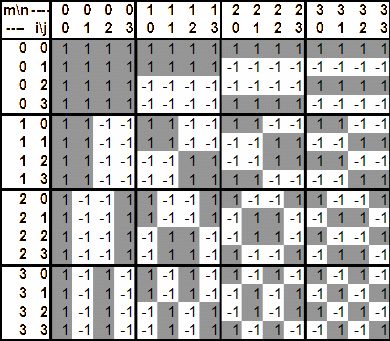
The transformation (8) is necessary to obtain a proper ordering of the Walsh functions to allow for calculating projections into the four main symmetries (vertical, horizontal, centro-symmetric or diagonal, and a double symmetry). The symmetries are as follows. If m is odd and n is even W_m,n has a horizontal symmetry; if m is even and n odd W_m,n has a vertical symmetry; if both are odd W_m,n is centro-symmetric, and finally if both are even, W_m,n is double symmetric; W_0,0 is an exception [11]. Figure 1 shows the Walsh functions for M = 4. Grey colour represents +1, white represents −1.

The probability of each of the four types of symmetry (vertical, horizontal, central, and double symmetry) is then:

$P_k={\sum }_{(m,n)}{\left(a_{m,n}\right)}^2/\left({\sum }_{n=0}^{M-1}{\sum }_{m=0}^{M-1}{\left(a_{m,n}\right)}^2-{\left(a_{\mathrm{0,0}}\right)}^2\right)$ (9)

In (9) k = 1,…,4 denotes individual symmetries, and ∑_(m,n) denotes the summation over a particular symmetry (odd/even, even/odd, odd/odd, even/even). The probabilities satisfy the normalization condition:

${\sum }_{k=1}^4{P}_k=1$ (10)

Then Shannon’s formula $S=-1/2\sum P_k{\text{log}}_2{P}_k$can be applied. The 1/2 factor serves to normalize the symmetropy so that the maximum value is 1 (consistent with spatial entropy). The higher the symmetropy, the higher the pattern symmetry and the disorder of the pattern are. For a random pattern (randomly distributed black and white cells), the symmetropy is 1 [10].

Temporal correlations and hurst coefficient

The last considered measure is the persistence (or long-term correlations) of data. Again, to the author’s knowledge this measure has not been used to quantify the spatial dynamics of combat before. Normally, it is used to quantify long-term memory in time series; in this instance it is applied to the set of individuals in a crowd instead. The Hurst coefficient answers the question “How is the motion of an individual A related to the motion of an individual B?” The correlations can provide enriching insights into the underlying dynamics of the system in question. The correlations have been used in a variety of areas ranging from stock exchange data to genetics and geophysics [11].

The temporal correlations are described in terms of the Hurst coefficient H [12]. The Hurst coefficient is related to the root mean square deviations from a trend in a system. If $H=0\text{.}5$ the system dynamics are random (there is no connection between the behaviour at two different points). If $H>0\text{.}5$ the system is correlated, and an occurrence of a particular behaviour suggests a similar tendency nearby. On the other hand, if $H<0\text{.}5$ the system is anti-correlated, so that an occurrence of extreme behaviour suggests an opposite extreme nearby.

A method called detrended functional analysis (DFA), developed by Peng et al [13], is commonly used to calculate the Hurst coefficient. It has been successfully applied in a variety of areas including physics, biology, and economies. DFA was designed specifically to deal with trends in nonlinear data. For instance, variations in stock indices are composed of two parts. One is a small long-term increase; the other is the deviation from this trend. To analyse long-term correlations in the deviations, the trend is removed first. The DFA is based on the root mean square analysis of a random walk and can be briefly summarized as follows [14].

To begin, it is assumed that there is a set {y₁ … y_m} of m measurements taken at points {x₁ … x_m}. First, the set is divided into m/n intervals (boxes) of length n (n = 1…m). Next, a least-square fit is performed on (x_j,y_j) pairs in each box. Next, for each box, the root-mean-squared deviation DF(n) of the data from the local trend is calculated as a function of the box size n. Then the values of DF(n) are averaged over all of the boxes to calculate a representative F(n). This is repeated for all possible box sizes n. Finally, the log-log plot of deviation F(n) versus n is used to calculate the Hurst coefficient H (slope). To facilitate the least-square fit, it is beneficial to select values for n so that they are uniformly distributed in logarithmic space. Since the box size n is limited by the sample size (it cannot be larger than the overall sample size m), it is necessary to have a sufficiently large sample to obtain meaningful results.

The spatial correlations in velocity (speed and direction) can possibly provide additional insights into crowd dynamics. The correlations are calculated independently for each velocity component, whether in Cartesian coordinates or in some other coordinate system.

For a random group of people (like pedestrians on a street somewhere in a downtown area), the speed and direction of individuals is likely to be uncorrelated ($H\approx 0\text{.}5$). On the other hand, for marching troops or a demonstrating crowd, the motion would be correlated. Thus the Hurst coefficient for such systems would be greater than 0.5, and could be close to 1. $H<0\text{.}5$(anti-correlated crowd) would suggest that the crowd is more or less stationary, with the distance between individuals remaining almost the same. Generally, a crowd with the Hurst coefficient $H\ne 0\text{.}5$ would be moving in some kind of an organized state, and thus should be considered potentially dangerous. The desired outcome of a CCO would likely be $H\approx 0\text{.}5$, suggesting uncorrelated motion of individuals (dispersing crowd). However, an important consideration would be the influence of the terrain on the mobility. In some special cases (such as a narrow street), the retreating crowd could actually move in a correlated fashion (all of the people retreating in the same direction). In such a case the retreat could lead to a higher Hurst coefficient.

A caveat needs to be included at this point. The Hurst coefficient is only meaningful for large numbers of data points (at least hundreds or thousands of data points). This means that either a large number of entities must be modelled, or the scenario must be replicated a large number of times (or both).

The Hurst coefficient can be calculated for other variables, providing insight into the system dynamics. For instance, Hurst coefficient can provide information about the phase transitions and other critical phenomena in a system [15].

Examples of cmoes for ccos

Scenario

To test the usefulness of the proposed CMOEs for CCO modelling, an example of a crowd confrontation scenario was developed. All of the above-described measures except C-R entropy were tested.

The scenario tested was taken from a previous study that evaluated the effectiveness of two different types of non-lethal launchers for CCOs. The scenario assumed an unruly crowd of 300 people gathered to force its way to a government building. The crowd was composed of two main subgroups: the “herd”, composed of middle-aged and elderly men, women and children, and “gangs” composed of much more aggressive youths. The Blue force was tasked to disperse the crowd. The objective was to disperse the crowd with no casualties on either side [3,16].

Kinetic non-lethal launchers were the primary tools employed by BLUE to achieve the objectives. The condition for the dispersal was attrition-based to accommodate requirements of an interactive wargame that was used to provide a framework for the simulation. To disperse the herd 15% of the entire crowd needed to be incapacitated, and to disperse gangs 50% of gang members needed to be incapacitated. For demonstration purposes, three of the analysed options are presented in this paper.

The modelling itself was performed using an ABM called Map-Aware Non-Uniform Automata (MANA) developed by the New Zealand Defence Technology Agency [MANA]. Version 3.2.2 was used for the study.

Entropy

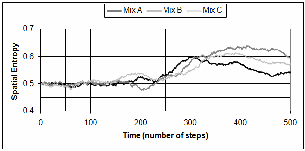
Figure 2 shows the temporal dependence of entropy for the CCO scenario. The crowd reached the Blue positions and began pushing against Blue around t = 100. Entropy did not change much until about t = 150, since until then there were not enough incapacitations to trigger a change in the crowd’s state. After about t ≈ 150 entropy began to change. For two of the options entropy slightly increased, while for one of the options it dropped. At about t = 220 the crowd dispersal actually started, which is reflected by the monotonous increase in entropy. Thus entropy provides a qualitative assessment of the crowd without the need for detailed knowledge of the causes of the change (incapacitations leading to dispersal in this instance).

The independence of spatial entropy from the factors causing dispersal permits its use as a characteristic of the crowd’s state that has a potential to incorporate impacts of a variety of factors on the crowd behaviour. Especially if ABMs were used, the state of dispersal could be affected by a range of influences such as warning shots, nearby incapacitations, incapacitations of a particular person(s), or fear of the Blue forces. Considering these additional factors would in turn allow for a more realistic modelling of crowd dynamics.

As mentioned above, there are small variations in entropy prior to the main increase caused by the crowd dispersal. Such occurrences of precursors is common in many dynamical systems (tremors preceding large earthquakes, pseudobreakups and field-line resonances preceding onset of a magnetospheric substorm [17,18]). The precursors typically serve as a warning for a larger event. It is also consistent with a subcritical system near a critical point (Discharge event systems) [19]. The occurrence of such precursors signalling major events could have significant practical use in combat.

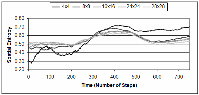
Thus, it seems clear that spatial entropy can be used to quantify combat dynamics in CCOs. One last word is needed about the dependence of entropy on the coarseness of the grid. Figure 3 shows the different shape of the entropy for the grids ranging from 4×4 subblocks to 28×28 subblocks. For the cases of more than 16×16 subblocks the variations in the entropy are small. In the former instances the subdivision is fine enough to allow for an average of less than a single crowd member per subblock. For coarse grids the results are rather sensitive to the number of subblocks. Especially for the grid of 4×4 subblocks there is a large spike in entropy at the beginning of the simulation. This spike is caused by the crowd moving from one subblock to another rather than by changes in the crowd dynamics. On the other hand the increase in the entropy due to actual dispersal is slightly delayed compared to finer grids. In this instance it is hard to distinguish between the artificial structures and the actual features due to the system dynamics. The best compromise appears to be the grid with the number of boxes approximately the same as the number of agents.

Fractal dimension

Like entropy, the fractal dimension was also calculated for the CCO scenario described earlier. The results are in Figure 4. While the crowd was advancing or confronting BLUE, the fractal dimension remained low. But once the crowd began to disperse, the fractal dimensions increased. After the period of increase a plateau was reached, with the maximum value approximately D_F = 1.5.

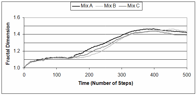
The maximum possible value of D_F for the crowd is related to the size of the area accessible to the crowd members. In the modelled scenario there was a significant portion of the area from which the crowd was to be kept out, plus a built-up area, thus restricting the range of values for D_F. The maximum value is easily estimated. The number of squares covering the entire battlefield is N₀ = (L/ε)². If the part of the battlefield with an area A is denied to the crowd, the number of the available squares is N = (L/ε)² × (1 – a), where a = A/(L/ε)². For the considered scenario about 55% of the terrain was available to the crowd (taking into account the area protected by BLUE and the buildings). That translates into the theoretical maximum value of D_F ~ 1.6. The maximum observed value was approximately 1.5, which corresponds well to the theoretical estimate.

Overall, the information obtained from the fractal dimension is similar to the information obtained from the spatial entropy. The main enhancement is that the magnitude of the fractal dimension provides information about the portion of the battlefield accessed by the crowd. This could be possibly used to measure mission success in situations that require restricting the crowd’s access to a certain portion of the battlefield (depending on whether the fractal dimension remains below D_FMAX or not).

Symmetropy

The results of symmetropy calculations for the CCO scenario are in Figure 5. The symmetropy provides the strongest signature of the state changes in the crowd at the dispersal point of all the CMOEs presented so far. There is a drop in the symmetropy (change in the system symmetries) as soon as the crowd begins dispersing. Once a majority of the crowd abandons the confrontation, the symmetropy begins increasing, and it reaches values around 1 as soon as the crowd is fully dispersed.

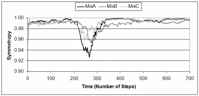
Like for entropy, there are precursors observable in the symmetropy during crowd dispersal. The variations are likely related to the different conditions for dispersal for the herd and the gangs. Overall, the symmetropy seems to provide a very efficient CMOE to characterize the crowd dynamics from the system point of view. As will be discussed later, the sudden changes in symmetropy may be connected with a phase transition-like phenomenon (criticality) in the crowd. The advantage of the symmetropy in identification of critical systems is that unlike the Hurst coefficient, it works also for sparse data.

Temporal correlations and hurst coefficient

Lastly, the Hurst coefficient was calculated. Since the crowd in the scenario consisted of only 300 individuals (not enough for the DFA), results from three replications were combined for the analysis. The results are in Figure 6. Combining results of several replications introduced extra variability in the data depending on the relative timings of events between replications. Despite the local variability, certain characteristics can still be derived. First, there was only a limited trend in the Hurst coefficient for the north-south direction. This was likely related to the fact that there was only a limited movement possible in this direction. In the east-west direction the trend is more interesting. This direction corresponds to the main flow of the crowd. The initial value of the Hurst coefficient was close to 0.5 (random). At about 100 steps it started increasing, with significant up and down variations possibly connected with more and more crowd members reaching and confronting Blue. At about 200 steps the value started decreasing, signifying crowd dispersal.

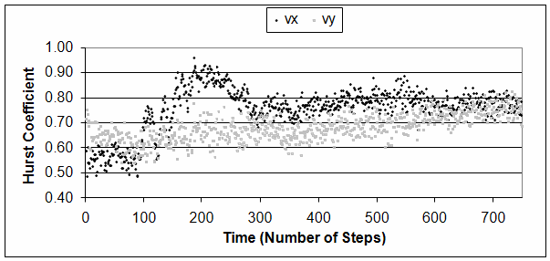
Overall, the trend in the Hurst coefficient for the east-west direction corresponds well to the dynamics observed in spatial entropy (including the precursors). Such changes in the Hurst coefficient reinforce the possibility of a phase transition-like phenomena in the crowd during the confrontation [15].

Phase transition in crowds

A crowd is a typical representative of complex adaptive systems (CAS). The crowd dynamics are governed by local rules and the interaction in the crowd is typically many on many. A crowd cannot be well decomposed into small crowds (or even to individuals), because the overall crowd dynamics are an emergent property of the entire system. The behaviour of a crowd changes (adapts) in response to external and internal factors (such as the presence and actions of law enforcement). As a result, no two crowds are exactly alike; yet in many cases the same dynamics are observed again and again. This similarity strongly suggests that the emergent dynamics are driven by similar mechanisms (akin to turbulence—while the details of molecular interactions differ, the turbulence has certain characteristics common across a wide range of situations). Following is a discussion of one such possible mechanism that might drive the emergent crowd behaviour.

Rapid, unidirectional change in the characteristics of a complex system (such as entropy, symmetropy or Hurst coefficient) typically characterizes the presence of a phase transition (criticality) in the system [15].

A special case of such a phase transition common in CAS’s is a self-organized criticality (SOC) [20]. A crowd reaching a criticality could have great implications on the overall system dynamics. It is likely that the entire crowd perception and internal dynamics would change. Furthermore, at the point of criticality the preferred scales in the system cease to exist, and the changes in the crowd behaviour (whether dispersal, or violent outbursts) would have an avalanche character, with sizes limited only by the overall size of the crowd.

Since a criticality in a crowd is likely to be an SOC, a brief summary of what SOC is included. The concept of SOC was first used to explain the commonalities in the dynamics of earthquakes for different faults. Since then it was used in a variety of fields ranging from seismology, space physics, and modelling of forest fires to description of international conflicts. SOC is an attractor for many complex systems, which means that the system will converge to this state no matter what the initial conditions are [20]. As is mentioned above, a system near a critical point is prone to avalanche-like character that reaches across all of the system scales. There is a power-law relationship between the size and frequency of the events.

The textbook example of a SOC is sand-piles [21]. Sand is slowly added to a pile. As the pile grows, the sand begins rolling down. Eventually, a stationary (but not static) state is reached, when on average the same amount of sand rolls off as it is added to the pile. The avalanche size and frequency are not causally related to the trigger that starts the avalanche, but are global system characteristics, and obey the power-law relationship between the size and frequency. Adding a single grain can in some instances trigger a large avalanche (perhaps even collapsing the pile), while in another case adding many grains may cause no change.

There is a relationship between the entropy and the correlations [22]. At the point of a dynamical phase transition both of these quantities should therefore feature an observable change. In the above scenario, both entropy and the Hurst coefficient show a similar dynamics. Between 100 and 150 steps the systems shows a beginning of dynamical changes (precursors). The correlations in the system increase across the crowd. The correlated system is consistent with the presence of a SOC in the system. Around 200 steps the system dynamics changes again, the Hurst coefficient begins decreasing (since more and more crowd members leave), while entropy increases showing that the crowd is dispersing. Once the entire crowd disperses (changes phase), the criticality is over (corresponding to an entire sand-pile collapsing).

At the point of the change in the trend for the Hurst coefficient the structure of the crowd changes with significant portions of the crowd bent on dispersal. This is further attested by the changes in symmetropy. Around the same time as the Hurst coefficient reaches its peak, the symmetropy drops suddenly (significant increase in the symmetry of the system). Similar changes were shown to be characteristic for the SOC in sand piles [10].

To summarize, the crowd dynamics at the point of dispersal appears to be consistent with the case of a SOC. However, more work is required to confirm the presence of a SOC in CCOs.

Summary and conclusions

The attrition provides only a limited means of quantifying CCOs, and other types of engagements in which the attrition plays a secondary role or is undesirable. The possibility of an alternative set of MOEs based on the complexity theory was investigated. The advantage of these complexity-based MOEs over more traditional measures is threefold. First, they are independent of attrition and therefore can provide means of assessment of outcomes of simulations even in the absence of attrition. Second, they characterize the temporal dynamics of the system during an entire simulation, rather than focusing on the end state. Thirdly, they provide good insights into the complexity of military operations that would be impossible using only traditional measures.

These complexity-based MOEs are meant as a supplement to traditional attrition-based MOEs that are being used in combat modelling to enhance the understanding of the system dynamics. The investigated MOEs are enumerated below:

• Shannon entropy: Carvalho-Rodriguez and spatial entropy were considered. C-R entropy is attrition-based, and therefore faces many of the same limitations as the traditional attrition-based measures. On the other hand spatial entropy provides valuable insights into the spatial dynamics on the battlefield. In the case of CCO it allows for the identification of the crowd dispersal independently of attrition.
• Fractal dimension: The box-counting dimension is used to characterize spatial distribution of crowd members. While similar to spatial entropy, it allows also the identification of the area of battlefield that was denied to the crowd.
• Symmetropy: Characterizes the symmetries and disorder in a dynamical system. Can be a very powerful tool in identification of spatial patterns. It can be also used to identify a presence of critical points in the system dynamics.
• Hurst coefficient: It is a measure of the correlations in the movement patterns of different crowd members. It also allows for identification of phase transitions in dynamical systems, and as such could be possibly used to identify significant system-wide changes in CCOs.

An example of calculations of these MOEs for a CCO scenario originally developed to assess non-lethal system effectiveness was presented to demonstrate the practicality of their use. The proposed MOEs proved to be very effective in describing the temporal changes of the crowd dynamics and allowed for a clear distinction between an advancing, structured crowd, and a dispersing crowd. The time of dispersal was generally easy to identify.

In the particular scenario used as a test-bed for the study, the CMOEs revealed the presence of a phase transition-like (critical) behaviour in the system. It is likely that the criticality observe is a case of self-organized criticality, typical for CAS. Entropy, Hurst coefficient and in particular symmetropy all hinted at this possibility. However, at this stage it is premature to make a conclusive statement about the presence of the SOC in the system. More work needs to be done in this area, which is beyond the scope of this paper.

Overall, the set of assessed complexity-based MOEs demonstrated their effectiveness in capturing crowd dynamics, and in identification of potentially important aspects of the confrontation (identification of a criticality).

The proposed CMOEs can be also used in the case of more traditional force-on-force combat models. In such an instance, they will provide quantitative information about force dynamics, and manoeuvres. They can also provide information about patterns in other measured quantities (including attrition), or about the long-term characteristics of measured quantities.

References

Author

Peter Dobias has received his MSc degree in theoretical physics from the Comenius University, Bratislava, Slovakia and his PhD in physics from the University of Alberta in Edmonton, Alberta, Canada. Currently he works at Defence R&D Canada Centre for Operational Research and Analysis. His main focus is combat modeling and wargaming of Land Force operations. He can be contacted by email at peter.dobias@drdc-rddc.gc.ca, or by phone at +1-613-992-4718 or fax at +1-613-992-5230.

References

[1] A. Ilachinski, Artificial War: Multiagent-based simulation of combat, World Scientific, 2004
[2] M. Herman, Entropy-Based Warfare, Booz-Allen & Hamilton, 1997
[3] P. Dobias, “Military Operations Involving Crowds: Agent-Based Modeling Using MANA and Non-Attrition-Based Assessment of Results”, in: Proceedings of 24th International Symposium on Military Research, Hampshire, UK, 2007
[4] M.K. Lauren and R.T. Stephen, “Fractals and Combat Modeling: Using MANA to Explore the Role of Entropy in Complexity Science”, Fractals, Vol. 10, No. 4, 2002, pp. 481-489
[5] G.C. McIntosh, D.P. Galligan, M.A. Anderson, and M.K. Lauren, MANA (Map Aware Non-Uniform Automata) Version 4 User Manual, DTA Technical Note 2007/3, NR 1465, 2007
[6] M.K. Lauren, G.C. McIntosh, N. Perry, and J. Moffat, “Art of War Hidden in Kolmogorov’s Equations”, Chaos, Vol. 17, No. 1, 2007, pp. 013121-013126
[7] F. Carvalho Rodrigues, “A Proposed Entropy Measure for Assessing Combat Degradation”, Journal of Operational Research Society, Vol. 40, No. 8, 1989, pp. 789-793
[8] P. Dexter, “Combat Entropy as a Measure of Effectiveness”, Journal of Battlefield Technology, Vol. 5, No. 3, 2003, pp. 33-39
[9] C.E. Shannon and W. Weaver, The Mathematical Theory of Communication, Univ. Illinois Press, Urbana, Illinois, 1949
[10] K. Nanjo, H. Nagahama, and E. Yodogawa, “Symmetropy and Self-Organized Criticality”, Forma, Vol. 16, No. 3, 2001, pp. 213-224
[11] D.D. Sornette, Critical Phenomena in Natural Sciences: Chaos, Fractals, Selforganization and Disorder: Concepts and Tools, Springer-Verlag, New York, 2nd ed., 2004
[12] H.E. Hurst, “Long-term Storage Capacity of Reservoirs”, Transmissions of American Society of Civil Engineers, Vol. 116, 1951, pp. 770-808
[13] C.-K. Peng, S.V. Buldyrev, S. Havlin, M. Simons, H.E. Stanley, and A.L. Goldberger, “Mosaic Organization of DNA Nucleotides”, Physics Review E, Vol. 49, No. 2, 1994, pp. 1685-1689
[14] J.A. Wanliss, “Nonlinear Variability of SYM-H Over Two Solar Cycles”, Earth, Planets, Space, Vol. 56, 2004, pp. 13-16
[15] J.A. Wanliss and P. Dobias, “Space Storm as a Dynamic Phase Transition”, Journal of Atmospheric and Solar-Terrestrial Physics, Vol 69, No. 6, 2007, pp. 675-684
[16] P. Dobias, Z. Bouayed, G. Woodill, and S. Bassindale, Optimum Number of Non-Lethal Weapon Launchers Study, Nickel Abeyance II: Non-Interactive Modeling Using MANA, DRDC CORA TR 2006-18, November 2006
[17] J.C. Samson, R. Rankin, and V.T. Tikhonchuk, “Optical Signatures of Auroral Arcs Produced by Field Line Resonances; Comparison with Satellite Observations and Modeling”, Annales Geophysica, Vol. 21, No. 4, 2003, pp. 933-945
[18] I.O. Voronkov, E.F. Donovan, P. Dobias, V.I. Prosolin, M. Jankowska, and J.C. Samson, “Late Growth Phase and Breakup in the Near-Earth Plasma Sheet,” in: Proceedings of the 7th International Conference on Substorms, eds. N. Ganushkina, T. Pulkinnen, Finish Meteorological Institute, 2004, pp. 140
[19] R. Woodard, D.E. Newman, R. Sanchez, and B.A. Carreras, “Persistent Dynamic Correlations in Self-Organized Critical Systems Away from Their Critical Point”, Physica A, Vol. 373, 2006, pp. 215-230, doi:10.1016
[20] P. Bak and K. Chen, “Self-Organized Criticality”, Scientific American, Vol. 264, No. 1, 1991, pp. 46-53
[21] P. Bak, C. Tang, and K. Wiesenfield, “Self-organized criticality: An Explanation of 1/f Noise”, Physics Review Letters, Vol. 59, No. 4, 1987, pp. 381-384.
[22] R.B. Griffiths, “Rigorous Results and Theorems”, in: Phase Transitions and Critical Phenomena, eds. Domb and Green, Academic Press, Vol. 140, 1972