
Volume 11, Number 1, March 2008
High-Fidelity Infrared Signature Modelling Using MATLAB Virtual Reality Toolbox
- 1 Department of Aerospace, Power & Sensors, Cranfield University at the Defence Academy of the United Kingdom, Shrivenham, SN6 8LA, United Kingdom.
Abstract
In light of the increasing terrorist surface-to-air missile (SAM) threat to civil and military aircraft, there is a continuing need for a high-fidelity, low-cost, PC-based, infrared (IR) signature scene modelling and simulation capability which could be used for development, testing, and evaluation of IR systems. An IR signature simulator has been developed utilizing the MATLAB Virtual Reality Toolbox software with the ability to adapt to rapidly changing tactical environments. It can model the IR signature of military targets in a 3D environment with special effects.
Introduction
The advancements in the computational capabilities of personal computers (PCs) has been so rapid that a job which a few years ago, was difficult for the expensive high-end proprietary workstations to perform, can now be done easily by a low-cost PC [1]. The military simulation community has taken advantage of this trend and has developed low-cost, PC-based, high-fidelity simulators for military applications.
Fidelity of the model
In the application of developing a computer model to simulate infrared (IR) scenes, the word “fidelity” has the twofold meaning: “accuracy” and “realism”. The accuracy relates to the mathematical modelling and means how close or truthful the results are to any measured readings. Whereas the realism relates to the appearance of correctness within the image presented. This essentially means how close to actuality or how realistic the scene looks, if compared with the actual scene and that any operator is convinced by what they see. The fidelity of the model depends upon the intended use. Low-fidelity models are simple and easy to use. On the other hand, the introduction of progressively more detail, leading to higher fidelity, has an obvious consequence on computational run time and operator expertise in running the simulation. High-fidelity models usually contain highly detailed terrains, man-made structures, atmospheric effects, detailed target geometry and thermal signature models. To make the model more realistic, the “special effects” such as the exhaust gas plume, dust, smoke, and clouds are added in these models.
High-fidelity simulators developed
Many military simulator developers have provided an integrated IR/electro-optical (EO), three-dimensional (3D) modelling environment. The following are a few examples of such systems [source internet]:
- Real-time IR/EO Scene Simulator (RISS) of Amherst Systems Inc., Northrop Grumman, New York, USA.
- Tactical Engagement Simulation Software (TESS) developed by Tactical Technologies Inc. Ontario, Canada [2].
- IR Target Generator (IRTG) and Target IR Simulator (TIRS) of CI Institute CA, USA.
- IR Scene Projector (IRSP) of Dynetics Alabama, USA.
- Aerial Target IR Simulator and Naval Target and Countermeasures Simulator (NTCS) developed by W.R. Davis Engineering Ltd. Ottawa, Ontaria, Canada [3].
- Vega Prime IR Scene developed by MultiGen-Paradigm, CA, USA.
- IR Scene Generator of Raytheon Missile Systems USA.
- Multi-Service Electro-optics Signature Code (MuSES) and PRISM of ThermoAnalytics, Inc., USA.
- Cameo-Sim broad scene simulator developed under DSTL (UK) MoD.
- Sensor-Vision is terrain visualization tool developed by MultiGen-Paradigm CA, USA.
- SIMTERM is a PC based computer simulator of thermal imagers developed by Inframet Inc., USA.
- CounterSim is an aircraft decoy assessment model (ADAM) developed by Chemring Countermeasures, High Post, UK.
- NATO Infrared Air Target Model (NIRATAM) and NATO’s NPLUME [4].
- DSTL(UK) Fly-in 2000 simulates the engagement of an aircraft, equipped with IRCM, by a missile with an imaging IR seeker [5].
The aim of this work is therefore to develop an adaptable and versatile IR signature modelling system, to run on any low-cost PC (with preferably no modification), using the powerful functions and routines available in MATLAB, to render scenes of sufficient realism as to convince a military operator that the image is “fit for purpose” in as near to real-time as possible.
IR signature modelling
All objects emit energy in the IR portion of the electromagnetic spectrum. The energy radiated from any object depends upon its property to absorb, reflect and transmit radiation. The temperature of the body and emissivity of the surface are the two dominant factors for IR signature modelling. The IR energy attenuates as it passes through the atmosphere. The IR energy received at the detector comprises of radiation from the target and background and reflected energy from other sources.
Developing the 3d virtual world
The IR signature scene has been visualized in the 3D scenario. The development of a 3D scenario starts with a story board in which the key features (such as the targets, missile, flares and background) are built and placed at appropriate locations in world coordinates. For simulation a plan script is written and animation sequences are developed. The viewpoints are selected for analysing the scene from different aspects. In this work, the tool used for development of the 3D virtual world is V-Realm builderTM which was provided with MATLAB Virtual Reality Toolbox.
Infrared radiations
The basic building element, on which all other radiometric quantities are based, is the spectral radiance. It is the radiant flux per unit area, per unit solid angle, and per unit bandwidth of wavelength. Assuming that the object is a Lambertian radiator, its radiance (N) can be evaluated from a simple modification to Planck’s Radiation Law [6]. The total radiance within a spectral band is found by integrating the radiance over the appropriate wavelength [7].
where:
N is the radiance, Wm-2sr–1.
λ wavelength in μm where λ1 and λ2 represent the spectral limits.
c1 first radiation constant, 3.7418×10⁸ Wm-2μm–1.
c2 second radiation constant, 1.4388×10⁴ μmK.
T absolute temperature of object, Kelvin.
eλ spectral emissivity of the object.
Sources of radiation
In any IR seeker missile or imaging system, the main sources of radiation are the targets and the backgrounds. Most military targets of interest are man-made sources. Typical military targets are aircraft, tanks, ships, and helicopters. These are made up of several materials. On a target, the IR signature appears as a series of hotter and colder regions. The targets can be modelled as one uniform temperature object or with different temperature zones or sub-targets. The sources of radiation on military targets are mainly the hot engine parts and the exhaust plume and the high-emissivity metal skin. Figure shows the various sources of radiation on an aircraft. Other dominant sources can be natural sources such as the sun, moon, skylight and star light. The solar irradiance on a target surface changes with a diurnal cycle. Also, the earth, sky and clouds can provide thermal emission and solar reflections.
Calculating radiance of the target
The target can be discretised/segmented into sub-targets using apparent temperature, emissivity, or material type, and the radiance of each target or sub-target is calculated, assuming that it radiates uniformly in all directions, using Planck’s law in (1). The target radiance values calculated at every 0.01 micron step are multiplied by the atmospheric transmittance (τa) calculated at every 0.01 micron step (0.01 micron steps have been chosen as a compromise between computational run time and spectral fidelity). The atmospheric transmittance is calculated using LOWTRAN atmospheric transmittance code [8]. The total radiance over the entire waveband of the detector is calculated as:
where:
Ntgττa is the total radiance after atmospheric attenuation
n is the number of 0.01 micron intervals in the detector waveband.
is the target radiance at every 0.01 micron interval.
is the atmospheric transmission at every 0.01 micron interval.
Adding reflection effects to the model
Other than the emissive properties of the targets, their reflective characteristics also contribute to the overall radiance received at the detector. The environmental sources of reflected radiation are the sun, the earth, the sky, atmosphere and clouds. Figure 1 shows the typical IR signature elements of an aircraft. Also, in the case of ground or sea targets, the inter-reflections caused by other targets in close vicinity may also contribute towards the overall radiance. However, in the case of airborne targets this may be neglected as aircraft are usually not very close to each other. The total radiance due to the reflections from other sources may be calculated as [9]:
![IR signature elements of an aircraft (Source [9]).](/journals/journal-of-battlefield-technology/volume-11/issue-01/assets/11-1-6-baqar/figures/figure01.gif)
where:
Nreflected is the total spectral radiance due to reflection.
Nss is the reflected sunshine.
Nes is either reflected earth shine or cloud shine.
Nsky is either reflected sky shine or cloud shine.
Ninref is reflected other targets shine or inter-reflections.
To calculate the total radiance due to reflections, the solar irradiance, earth and sky irradiance are first calculated. The radiance due to reflections depends upon the relative position of the sources, the viewers (seeker) and the angle which they make with the reflecting surface. The reflected radiance has two components, one due to the specular reflectivity and the other due to the diffused reflectivity (due to the scattering) [10]. Ideally, for true modelling of the physical process, the radiance due to both these components has to be calculated at every point in the scene. However, in the case of dynamic simulations where the position of the target and seeker are changing rapidly, calculating reflected radiance at every point may be computationally expensive. Therefore, to add the effects of reflections on the overall IR signature, an alternate approach has been used. This may be done by controlling the material properties (appearances) of the objects in virtual world modelling in VRML. The solar, earth, and sky irradiance may be modelled as independent sources and the “diffusedColor”, “ambientIntensity”, “ambientColor”, and “shininess” used to represent the radiant reflective properties of the material.
Modelling IR signature of the exhaust gas plume
The exhaust gas plume of an aircraft is a spectral emitter and is usually the dominant source of thermal radiation in the 3–5 micron band [11]. The body of a military target is generally solid metal and opaque in nature, whereas, the turbine engine exhaust gas plume comprises of the residue leftover from the combustion process and is non-opaque in nature. Thus the exhaust gas plume may be assumed to emit thermal radiation and transmit the energy through a non-opaque volume and any reflections may be neglected [11]. Therefore, the total radiance of the plume can be represented as:
where:
Ntotplume is the total radiance of the plume.
Nplumemis is the radiance due to emissive properties of plume.
Nbehindplume is the radiance of the object behind plume.
τplume is the transmittance of the plume.
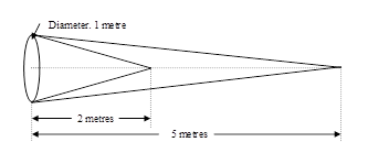
Equation (4) has two components, one Nplumemis that is the radiance due to emissive properties of plume. This is similar to the one which is also present in the case of opaque objects. But the other component due to the transmittance is the radiance of objects behind the plume (Nbehindplume) factored with the transmittance of the plume (τplume). The radiance behind the plume may be that of the target itself, the sky or other backgrounds and is dependant upon the target aspect or seeker’s viewing angle. Calculating the exhaust gas plume radiance is non-trivial. The shape and volume of the plume is not constant. Due to the fast movement of the aircraft and the presence of gases (such as CO2 and H2O) in the atmosphere, the plume is gradually diluted in the surrounding atmosphere and it is therefore difficult to draw a boundary between the plume and the atmosphere. However, for IR signature modelling purposes, the bulk of the radiation of the jet engine exhaust plume comes from the vicinity of the exit plane in a region called the inviscid core. Figure 2 shows the inviscid core behind the aircraft engine nozzle. As much as three-quarters of the total plume radiance may be generated within a length shorter than the structural length of the aircraft [11]. The region beyond the inviscid core emits more weakly and is more easily absorbed by the cool atmospheric gases. For IR signature modelling it is important to consider the shape, size and conditions of the hottest exhaust gas region. For a circular nozzle, the inviscid core may roughly be conical with the base area as that of the nozzle exit area and a length shorter than the aircraft length [11].
![Simplified aircraft jet engine exhaust plume (Source [11]).](/journals/journal-of-battlefield-technology/volume-11/issue-01/assets/11-1-6-baqar/figures/figure02.gif)
The inner cone representing a higher temperature as compared to the outer cone. In (4), the plume radiance due to the emissive properties (Nplumemis), for the entire waveband of the detector is calculated by first calculating the radiance at every 0.01 micron interval using (1) and then multiplying it with the atmospheric transmittance (τa) calculated at every 0.01 micron. The Nplumemisτa at every 0.01 micron is then summed to calculate to total spectral radiance of the plume due to emissivity.
where:
Nplumemisτa is the plume emissive radiance after atmospheric attenuation.
n is the number of 0.01 micron intervals in the detector waveband.
is the plume radiance due to emissivity at every 0.01 micron interval.
is the atmospheric transmittance at every 0.01 micron step.
The radiance due to the emissive properties of the plume (Nplumemis) may be represented as the “emissiveColour” in VRML. The other component of plume radiance due to the transmittance as shown in (4), may be calculated by multiplying the plume transmittance (τplume) with the radiance of the object behind the plume (Nbehindplume). However, in the VRML 3D virtual world, this could be modelled as the “transparency” field of VRML representing the plume transmittance (τplume) and the colour of the background is representing the radiance behind the plume (Nbehindplume). Assuming that the radiance due to reflection is negligible in the gaseous plume, then the value of the “transparency” may be calculated as:
where:
τplume is the transmittance of the plume, and
εplume is the total emissivity of the plume.
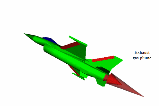
Figure 3 shows the 3D VRML model of the aircraft with an exhaust gas plume modelled at the back of the tail section as two semi-transparent co-centric cones.
Modelling appearance of sub-targets in virtual world
In the VRML file format, a 3D virtual world scene is described by a hierarchical tree structure of several objects. These objects are called “nodes”. A node may contain other nodes “child nodes” under it. When a new node is created, the required fields are automatically generated and filled with default values. These fields hold the data for each node. In VRML, every geometrical object contains an independent “geometry” node and “appearance” node [12]. The geometry node controls the size and shape of each part of the object. Whereas, the appearance node controls the texture and material properties. The appearance node specifies the physical properties such as the “ambientIntensity”, “diffusedColour”, “emissiveColour”, “shininess”, “specularColour” and “transparency”. These properties of each sub-part can be controlled independently. The radiances are then normalized over the range of the colour-map. A colour-map of different sizes can be used to map radiance data. The typical colour-indices are 128, 256, 512, or 1024.
where:
is the normalized radiance of sub-targets.
Nmax is the maximum value of radiance available in the scene.
Colour_ index is the number of indexed RGB colours in the colour-map.
The normalized radiance of each sub-target is then converted into the corresponding RGB colour value. The sub-targets are modelled in VRML as objects with different appearance. The material fields of each sub-target are altered to resemble their IR signature.
Table 1 summarizes the different material types and their corresponding appearance fields. Using these material properties, the IR signature of sub-targets with different radiometric properties are modelled in the 3–5 and 8–12 micron wavebands. The simulations are extensively carried out at different ranges and aspects.
Selecting “colour-map” to represent radiance values
In real life, the visible colours do not correspond to IR radiations (as the IR band is outside the visible spectrum). However, for realism the different values of radiance in the IR waveband may be represented as corresponding false colours. The predefined range of colours used to map an entire range of particular data values is called a “colour-map” [13]. Figure 4 shows different colour-maps which are supported by MATLAB. These colour-maps represent different ranges of colours.
![Different colour-maps supported by MATLAB ( Source[13]).](/journals/journal-of-battlefield-technology/volume-11/issue-01/assets/11-1-6-baqar/figures/figure04.gif)
Each of these thirteen colour-maps has been evaluated to see how they represent the radiance values in the two IR wavebands of 3–5 and 8–12 micron. The effect of the different colour-maps on the IR signature appearance is monitored by running the simulation several times. Assessment has been made on the visibility of the expected features in the IR scene (for example the visibility of the IR plume in the 3–5 micron region—see the results section and Table 9 for details). Some colour-maps do not effectively represent the IR signatures, whereas other colour-maps represent the IR signature scene more successfully.
Modelling IR background
Based on the missile-target engagement scenario, in an IR scene, the background may consist of one uniform background or a combination of different sub-backgrounds. For the air-to-ground mode, the background may be objects such as runways, buildings, ground, sand, woodland, hills etc or any combination of these. In the case of surface-to-air missile simulation, the background is typically the sky or clouds. Whereas, in the case of air-to-air missiles, depending upon the target and missile relative positions, the background may be either sky or ground or both (horizon). Therefore, depending upon the planned scenario, any type of background may be modelled accordingly. In VRML, there is a provision for the readymade “background” node that models the whole space around any scene as layers of sky in the upper hemisphere and layers of ground in the lower hemisphere. The colour and size of these layers can be controlled by the “groundAngle”, “groundColor”, “skyAngle”, and “skyAngle” fields [12]. The “background” node of VRML may possibly be used to model the IR background. The sky can be divided into three layers with two angles dividing the upper hemisphere. However, based on the desired fidelity, the number of layers of the sky may be increased or decreased accordingly. The colour of each layer corresponds to the sky radiance at selected altitudes. The sky-radiance data for a number of weather conditions and altitudes is generated by running the LOWTRAN atmospheric transmission code. Table 2 (radiance values) shows various inputs to be fed in to LOWTRAN for calculating the sky-radiance [8]. This table shows the three sets of inputs which may represent “good”, “typical”, and “bad” weather conditions.
However, the ground in the lower hemisphere is kept as one uniform layer. The radiance of the ground is calculated from the temperature and the emissivity using Planck’s Law—(1). The total radiance received at the detector is calculated after considering the atmospheric transmission (τa). Table 3 shows the typical values of the emissivity (total normal) and temperature of various background materials.
Transmission of infrared radiation through earth’s atmosphere
The energy radiated from the target or source has to pass through some medium before reaching the sensor. Generally this medium is the atmosphere. In the visible region, our ability to view a distant object is not constant and depends upon the weather conditions. Similarly, the IR sensors are adversely affected by the changing atmosphere. The influence of the atmosphere on thermal radiation is a complex process. The earth’s atmosphere is a mixture of many gases and the existence of these gases in the atmosphere varies with altitude, time, and space.
Atmospheric transmittance
The transmission of the atmosphere present between the scene and the sensor is calculated on the basis of the absorption, scattering and refractive-index fluctuations or turbulence. The turbulence in the atmosphere is due to the temperature, pressure and density in-homogeneities which may result in blurring and distortion of images. It is usually only noticeable when viewing small objects at long distances and has little effect on near objects [7]. The absorption and scattering are usually grouped together under the topic of extinction which causes attenuation in the amount of radiant flux passing through the atmosphere. The transmittance of a path through the atmosphere can be expressed as:
where:
τ represents the transmittance of the atmosphere.
σ is the extinction coefficient.
x is the path length of the atmosphere.
This principle is known as the Beer-Lambert Law [7]. Under most conditions the extinction coefficient (σ) is made up of two components:
where, α is the absorption coefficient and accounts for the absorption by the gas molecules of the atmosphere and γ is the scattering coefficient which accounts for scattering by small particles suspended in the atmosphere. In the IR region of the spectrum, absorption typically dominates atmospheric propagation and scattering can usually be ignored with limited impact on the results [14]. However, this approximation may not be applicable at the shortest IR wavelengths where some early IR missiles operate.
Atmospheric path-radiance
As the atmosphere comprises of particles, they thermally emit radiation along the path in the line-of-sight (LOS) of the source to the detector. The path-radiance of the atmosphere may be calculated by considering atmospheric particles as blackbodies at a particular temperature. The path-radiance becomes negligible as the path transmittance gets higher (closer to one). Therefore, with a cold clear sky, the path radiance can usually be neglected but at high temperatures it can cause noticeable effects. Similarly, the path radiance can be negligible for short path distances [7].
Modelling atmospheric effects on IR signature
In this work, the LOWTRAN atmospheric propagation code is used for modelling the atmospheric transmittance and the path radiance. By running LOWTRAN several times the transmittance data for different weather conditions and altitudes are calculated and stored in look-up tables as a function of wavelength. Table 2 (transmittance values) lists the typical LOWTRAN input parameters required to calculate the atmospheric transmission data [8]. By selecting different altitudes, path types, weather conditions and model atmosphere values, several sets of transmission data can be generated.
VRML vs IR comparison summary
The various “nodes” and “fields” of VRML may be used for modelling the IR signature scene. Table 4 summarizes the features of the IR signature modelling and the corresponding nodes and fields of VRML which may be used to model these features.
Test scenario setup
The IR signature of an aircraft is considered as a set of sub-targets for high-fidelity modelling. The appearance of the sub-targets in the IR waveband as per the radiometric properties is analysed. The leading-edge reflection, the exhaust gas plume and the cold-sky reflections from the canopy are analysed for their appearance in the virtual world. The radiance values are converted into a corresponding RGB colour-map. The IR signature of one static aircraft at 1,000-m altitude is analysed from the seeker of an air-to-air missile at the same altitude. The distance between the target and missile is kept as 750 m. The IR spectral bands of 3–5 and 8–12 micron are considered. The seeker is viewing the aircraft from the beam, tail, and nose aspects.
Missile input parameters
Type of Missile: Air-to-air
Detector Size: 0.3 mm
Image Size in pixels: 256 × 256 pixels
Spectral Band Coverage: 3–5 and 8–12 μm
Range between target and missile: 750 m
Background input parameters
Background upper Hemisphere: Three Layers of Sky
Altitude of layers: sea level, 1 km, 10 km
Distance from seeker: 0.75 km
Background lower Hemisphere: Ground
Temperature: 290 K
Emissivity: 0.9
Target input parameters
The sub-target temperatures and radiometric properties are shown in Table 5.
The inviscid core of the exhaust gas plume is modelled as co-centric cones. The dimensions of the cones are shown in Figure 5. The material field values for the sub-targets are shown in Table 6.
Results
The numerical values of the target and background radiance and the corresponding colour are given in Table 7 for the 3–5 micron waveband and the values for the 8–12 micron waveband are given in Table 8. The sub-targets I, II, III, IV and V mentioned in Table 5 and Table 6 correspond to the “body”, “nose”, “leading edges”, “tail-pipe” and “canopy” respectively. Similarly, the sky radiance I, II and III corresponds to sky layers at sea level, 1-km and 10-km altitudes respectively.
The output images captured for the 3–5 and 8–12 micron waveband from the beam aspect are shown in Figure 6. The same images of Figure 6, is recaptured without the background and is shown as Figure 7.
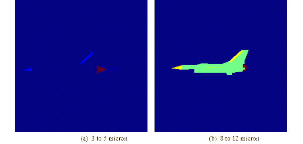
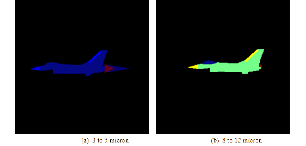
Figure 8 shows the effect of the reflections on the overall IR signature of the target in 3–5 micron waveband. The same is shown in Figure 9 but without the background.
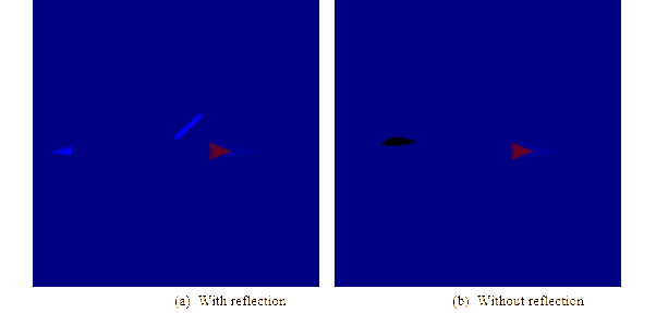
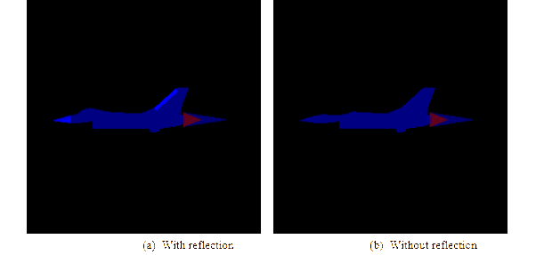
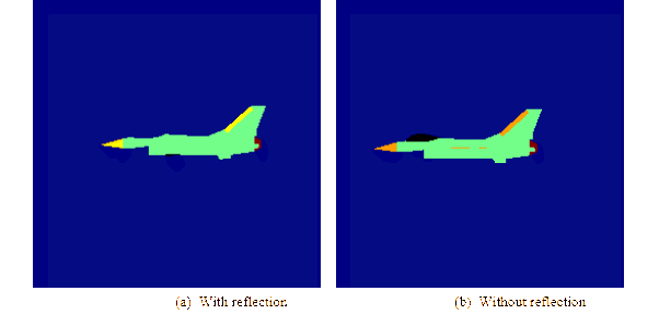
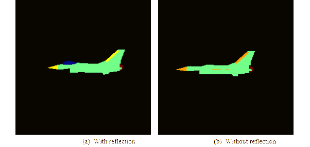
Figure 10 shows the reflection effects in 8–12 micron waveband. The same images but without the background are shown in Figure 11.
Different colour-maps have been tried to see how they represent the IR signature scene in 3–5 and 8–12 micron wavebands. The 2D images of the IR scene with these different colour-maps have been observed and Table 9 summarizes the visual effects.
Discussion on results
The results generated using the test scenario are analysed for the appearance of the IR signature representation in virtual reality and are discussed in the following paragraphs.
Different colour-map
On the basis of the results observed and the summary shown in Table 9, it is suggested that the “Jet” colour-map is the most suitable to represent the IR signatures in both the 3–5 and 8–12 micron bands. Also this colour-map shows the leading-edge reflections and the canopy cold sky reflections.
The “Summer” colour-map may also be used to represent the IR signature in the 3–5 and 8–12 micron wavebands but this reproduction is not quite as good as the “Jet” colour-map.
The “Cool” colour-map may be used to represent the 8–12 micron waveband but this is not very clear in the 3–5 micron waveband. The “Hot” colour-map may be used to represent the 3–5 micron waveband reasonably well, but this is not realistic in the 8–12 micron waveband. The “Gray”, “Bone”, and “HSV” could not show the reflection effects.
Physical properties vs material properties of VRML
The emissivity, reflectivity and transmissivity of the objects in the IR waveband may be related to the material properties of the objects in the virtual reality. The emissivity and temperature represent radiance which may be shown by “emissiveColor” in VRML. The reflectivity is modelled by the “diffuseColor” and the “specularColor” along with the “ambientIntensity” field of the material properties. The transmissivity is represented by the “transparency” field of VRML. Table summarizes the suggestions for representing the IR signature of the different types of material in the virtual world. The different possibilities of material properties in VRML are tried and finally on the basis of visual appearance a strategy is suggested to represent the IR signature of a scene in the virtual reality. The summary of this option is given as under:
- Dull Metallic Body. The dull metallic body or surface may be shown as “emissiveColor” in VRML.
- Gaseous Plume. The exhaust gas plume of the aircraft may be shown as “emissiveColor” with “transparency” representing the transmissive nature of the gaseous plume.
- Shining Leading-edges. The leading-edges of the aircraft may be modelled as “emissiveColor”, “diffuseColor” with “ambienrtIntensity”, and “specularColor” with “shininess”.
- Cold Sky Reflections. The cold sky reflection effects from the glass canopy depend upon the emissivity and reflectivity of the glass. The radiance of the canopy may be shown as “emissiveColor” and the sky radiance may be shown as the “specularColor” along with “ambienrtIntensity” and “shininess” to represent the reflection of the sky from the canopy.
Plume radiance
From Figure 6 and Figure 7, the exhaust gas plume of the aircraft is the dominant source of radiation in the 3–5 micron waveband. Whereas, in the 8–12 micron waveband the signatures of the plume are negligible as the spectral emissivity of the plume is almost zero.
Cold sky reflection from canopy
In the case of the canopy, out of the three physical properties, the transmittance is neglected and only the effects due to emissive and reflective component are considered. The emissive component may cover the radiance of the canopy material and is shown as “emissiveColor”. The reflective part may be covered by using “specularColor” corresponding to the radiance of the sky with “shininess” as reflectivity. But there is no “diffuseColor” on the canopy. To make sky reflections prominent an additional light source may be modelled to represent the sky or sun irradiance. Figures 8 to Figure 11 shows the IR signature of a target aircraft with and without cold sky reflection effects in the two IR wavebands of the 3–5 and the 8–12 micron.
Further work
At present, only the atmospheric attenuation is considered for calculating the total radiance. As the atmosphere comprises of particles, they thermally emit radiation along the path in the LOS from the source to the detector. Hence for higher order modelling, the path-radiance component Npath(λ) may be added to the total radiance. Therefore, the total spectral radiance received at the detector can be calculated as:
where:
Ntotal(λ) is the radiance after atmospheric attenuation.
Nsource(λ) is the radiance of the object.
τpath(λ) is the atmospheric transmittance of the path length in between.
Npath(λ) is the path-radiance.
The path-radiance becomes less dominant as the path transmittance gets higher (closer to 1). Therefore, for the case of the cold clear sky, the path-radiance may contribute less towards the total radiance. However, at high atmospheric temperatures or low atmospheric transmittance values, the path-radiance may contribute significantly towards the total radiance. Similarly, the path-radiance can be less significant for shorter path lengths as compared to longer paths. A possible approach for considering the path-radiance (Npath) effects may be to calculate the path-radiance using LOWTRAN, but to cater for the changing distance between the target and the sensor during simulation, the path-radiance needs to be calculated for changing path length at every time interval or frame. This could possibly be done by running the LOWTRAN code several times for different path lengths and storing the data sets into lookup tables.
Conclusion
The low-cost PC based high-fidelity IR signature scene model has been developed. The high-fidelity physics based IR signature of military targets and backgrounds are modelled. The models are based on the equations derived from open-source material and published literature. The atmospheric conditions such as “good”, “typical” or “bad” weather conditions are considered to model atmospheric transmission and the sky radiance. The realistic 3D models of sub-targets with different temperature zones and radiometric properties are developed to represent dull metallic body parts, shining leading edges, hot exhaust gas plumes and reflecting canopies. These effects are modelled using MATLAB Virtual Reality toolbox.
| Material Type | Aircraft Part | Ambient Intensity | Diffuse Colour | Emissive Colour | Shininess | Specular Colour | Transparency |
|---|---|---|---|---|---|---|---|
| Dull Metal | Body | 0 | 0 | Body Radiance | 0 | 0 | 0 |
| Exhaust Nozzle | 0 | 0 | Nozzle Radiance | 0 | 0 | 0 | |
| Engine Intake | 0 | 0 | Engine Intake Radiance | 0 | 0 | 0 | |
| Shining Metal | Nose | 1.0 to 0.5 | Nose Radiance | Nose Radiance | 1-emissivity | Nose Radiance | 0 |
| Leading Edges | 1.0 to 0.5 | Leading Edges Radiance | Leading Edges Radiance | 1-emissivity | Leading Edges Radiance | 0 | |
| Hot Gases | Exhaust Plume | 0 | 0 | Plume Radiance | 0 | 0 | 1-emissivity |
| Glass | Canopy | 1.0 | 0 | Canopy Radiance | 1-emissivity | Sky Radiance | 0 |
| PARAMETER/ATMOSPHERE TYPE | GOOD | TYPICAL | BAD |
|---|---|---|---|
| MODEL ATMOSPHERE | 1976 US Standard | ||
| TYPE OF ATMOSPHERIC PATH | Horizontal Path | ||
| MODE OF EXECUTION | Radiance | Transmittance | |
| EXECUTED WITH MULTIPLE SCATTERING | No | ||
| AEROSOL MODEL USED | No aerosol attenuation | Rural-Visibility = 23 km | Rural-Visibility = 5 km |
| UPPER ATMOSPHERE AEROSOLS | Background Stratospheric | ||
| CLOUD/RAIN AEROSOL EXTENSIONS | No Cloud or Rain | No Cloud or Rain | Cumulus Clouds |
| RAIN RATE (mm/hour) | 0 | 0 | 2 mm/hour |
| GROUND ALT ABOVE SEA LEVEL (km) | 0 | ||
| INITIAL ALTITUDE (km) | 0 | 1 | |
| FINAL ALTITUDE (km) | 0 | 1 | |
| INITIAL ZENITH ANGLE (degrees) | 0 | ||
| PATH LENGTH (km) | 200 | 1 | |
| SHORT PATH-0/ LONG PATH-1 | 1 | 0 | |
| INITIAL FREQUENCY in wavenumber | 665 (15.038 micron) | ||
| FINAL FREQUENCY in wavenumber | 10000 (1 micron) | ||
| FREQUENCY INCREMENT in wavenumber | 5 (0.01 micron) | ||
| NUMBER ON PLOTS | 1 | ||
| HARD COPY OPTION | 1-generate print / printer output | ||
| INTERACTIVE GRAPHICS MODE | 6- 640x350 dot Mode | ||
| PLOT TYPE | 0-Radiance | 2-Transmittance | |
| LENGTH OF X-AXIS (in inches) | 7 | ||
| BEGINNING WAVENUMBER/wavelength (µm) | 665/1.00 | ||
| ENDING WAVENUMBER/wavelength (µm) | 10000/15.00 | ||
| LENGTH OF Y-AXIS (in inches) | 6 | ||
| MINIMUM RADIANCE/TRANSMITTANCE | 0 | ||
| MAXIMUM RADIANCE/TRANSMITTANCE | 1 | ||
| Y-Axis Annotation Interval | 0.1 | ||
| LINE TYPE | 1 (normal line) |
| Material | Emissivity | Temperature (K) |
|---|---|---|
| Red Brick | 0.93 | 293.15 |
| Concrete | 0.92 | 293.15 |
| Sand | 0.90 | 293.15 |
| Wood (planed Oak) | 0.90 | 293.15 |
| Water (distilled) | 0.96 | 293.15 |
| Snow | 0.85 | 263.15 |
| IR Signature Scene | VRML Nodes and Fields | Remarks |
|---|---|---|
| Shape of objects | “geometry” nodes | Any 3D shape may be modelled using different geometrical shapes |
| Size of objects | “scale” | Size of an objects may be chaged as per requirements |
| Objects with same radiometric properties | “DFE” and “USE” node | Plan one “DFE” node (short of “define” to define a name for a node) in the start and call it for different objects by “USE” node |
| Landmarks, hills (terrain) | “elevationGrid” node | Irregular terrain may be modelled using elevation grid |
| Sky and ground as background | “background” node | Multi-layer sky and uniform ground may be modelled |
| Temperature and emissivity | “emissiveColour” field | Radiance of objects may be modelled as fake colours |
| Reflectivity (sun shine, earth shine, sky shine) | “ambientIntensity” “shininess” “specularColour” and light source | The leading-edge reflections and cold-sky reflections may be modelled |
| Transmissivity | “transparency”, “emissiveColour” and background colour | Exhaust gas plume, clouds, smoke etc. may be modelled using transparency |
| Part | Emissivity | Reflectivity | Transmittance | Temperature |
|---|---|---|---|---|
| Body | 0.9 | 0.1 | 0.0 | 320 K |
| Nose | 0.9 | 0.1 | 0.0 | 350 K |
| Leading Edges | 0.9 | 0.1 | 0.0 | 350 K |
| Tail pipe | 0.9 | 0.1 | 0.0 | 380 K |
| Canopy | 0.5 | 0.5 | 0.0 | 250 K |
| Plume inner | Spectral | 0.0 | 0.5 | 1000 K |
| Plume outer | Spectral | 0.0 | 0.5 | 500 K |
| Sub-Target | Ambient Intensity | Diffuse Color | Emissive Color | Shininess | Specular Color | Transparency |
|---|---|---|---|---|---|---|
| Body | 0 | 0 | Nbody | 0 | 0 | 0 |
| Nose | 0.5 | Nnose | Nnose | 0.8 | Nnose | 0 |
| Leading Edges | 1.0 | Nedge | Nedge | 0.1 | Nedge | 0 |
| Tail-pipe | 0 | 0 | Ntailpipe | 0 | 0 | 0 |
| Canopy | 1.0 | 0 | Ncanopy | 0.7 | Nsky | 0 |
| Exhaust Plume Inner | 0 | 0 | Nplminn | 0 | 0 | 0.5 |
| Exhaust Plume Outer | 0 | 0 | Nplmout | 0 | 0 | 0.5 |
| Variable | Units | Value I | Value II | Value III | Value IV | Value V |
|---|---|---|---|---|---|---|
| Background Total Radiance | W m-2 sr-1 | 1.1601 | ||||
| Background Total Radiance after Attenuation | W m-2 sr-1 | 2.1774 x10⁻¹¹ | ||||
| Sky Total Radiance after Attenuation (three layers) | W m-2 sr-1 | 0.2232 x10⁻¹² | 0.1652 x10⁻¹² | 0.0020 x10⁻¹² | ||
| Sub-target Total Radiance (five sub-parts) | W m-2 sr-1 | 3.3372 | 8.0988 | 8.0988 | 17.2457 | 0.1092 |
| Sub-target Total Radiance after Attenuation | W m-2 sr-1 | 0.0701 x10⁻⁹ | 0.1845 x10⁻⁹ | 0.1845 x10⁻⁹ | 0.4171 x10⁻⁹ | 0.0016 x10⁻⁹ |
| Exhaust Gas Plume Total Radiance (two layers) | W m-2 sr-1 | 748.619 | 24.4882 | |||
| Exhaust Gas Plume Radiance after Attenuation | W m-2 sr-1 | 0.2711 x10⁻⁷ | 0.0071 x10⁻⁷ | |||
| Maximum Radiance | W m-2 sr-1 | 0.2711 x10⁻⁷ | ||||
| Normalizing Factor | 9.4424 x10+9 | |||||
| Normalized Radiance Background | 0.2056 | |||||
| Normalized Radiance Sky | 0.0021 | 0.0016 | 0.0000 | |||
| Normalized Radiance Sub-target | 0.6616 | 1.7424 | 1.7424 | 3.9383 | 0.0155 | |
| Normalized Radiance Exhaust Gas Plume | 256 | 6.7154 | ||||
| Colour Background (RGB) | Red Green Blue | 0 0 0.5156 | ||||
| Colour Sky | Red Green Blue | 0 0 0.5156 | 0.0 0.0 0.5156 | 0.0 0.0 0.5156 | ||
| Colour Sub-targets | Red Green Blue | 0.0 0.0 0.5156 | 0.0 0.0 0.5315 | 0.0 0.0 0.5315 | 0.0 0.0 0.5625 | 0.0 0.0 0.5156 |
| Colour Exhaust Gas Plume | Red Green Blue | 0.5 0.0 0.0 | 0.0 0.0 0.6094 |
| Variable | Units | Value I | Value II | Value III | Value IV | Value V |
|---|---|---|---|---|---|---|
| Background Total Radiance | W m-2 sr-1 | 29.1956 | ||||
| Background Total Radiance after Attenuation | W m-2 sr-1 | 1.9188 x10⁻¹⁰ | ||||
| Sky Total Radiance after Attenuation (three layers) | W m-2 sr-1 | 0.2076 x10⁻¹¹ | 0.1836 x10⁻¹¹ | 0.0126 x10⁻¹¹ | ||
| Sub-target Total Radiance (five sub-parts) | W m-2 sr-1 | 47.0296 | 70.0883 | 70.0883 | 98.4048 | 7.2604 |
| Sub-target Total Radiance after Attenuation | W m-2 sr-1 | 0.3054 x10⁻⁹ | 0.4496 x10⁻⁹ | 0.4496 x10⁻⁹ | 0.6240 x10⁻⁹ | 0.0484 x10⁻⁹ |
| Exhaust Gas Plume Total Radiance (two layers) | W m-2 sr-1 | 0.0 | 0.0 | |||
| Exhaust Gas Plume Total Radiance after Attenuation | W m-2 sr-1 | 0.0 | 0.0 | |||
| Maximum Radiance | W m-2 sr-1 | 0.6240 x10⁻⁹ | ||||
| Normalizing Factor | 4.1025 x10+11 | |||||
| Normalized Radiance Background | 78.7174 | |||||
| Normalized Radiance Sky | 0.8517 | 0.7534 | 0.0518 | |||
| Normalized Radiance Sub-target | 125.269 | 184.447 | 184.447 | 256.000 | 19.8597 | |
| Normalized Radiance Exhaust Gas Plume | 0.0 | 0.0 | ||||
| Colour Background (RGB) | Red Green Blue | 0.0 0.7344 1.0000 | ||||
| Colour Sky | Red Green Blue | 0.0 0.0 0.5156 | 0.0 0.0 0.5156 | 0.0 0.0 0.5156 | ||
| Colour Sub-targets | Red Green Blue | 0.4531 1.000 0.5469 | 1.000 0.6250 0.0 | 1.000 0.6250 0.0 | 0.500 0.0 0.0 | 0.0 0.0 0.8125 |
| Colour Exhaust Gas Plume | Red Green Blue | 0.0 0.0 0.5156 | 0.0 0.0 0.5156 |
| Colour Map | 3–5 micron Band | Appearance | 8–12 micron Band | Appearance |
|---|---|---|---|---|
| HOT | Body: no contrast (OK) Edges: very dim reflection Canopy: no reflection Plume: good contrast | BAD | Body: good contrast Edges: low reflection Canopy: low reflection | BAD |
| JET | Body: no contrast (OK) Edges: good reflection Canopy: prominent reflection Plume: good contrast | GOOD | Body: visible Edges: prominent reflection Canopy: good reflection | GOOD |
| GRAY | Body: not visible Edges: no reflection Canopy: no reflection Plume: only inner vis | BAD | Body : visible Edges: good reflection Canopy: no reflection | BAD |
| BONE | Body: not visible Edges: no reflection Canopy: no reflection Plume: only inner vis | BAD | Body : visible Edges: good reflection Canopy: no reflection | BAD |
| HSV | Body: not visible Edges: no reflection Canopy: good reflection Plume: not good | BAD | Body: visible Edges : good reflection Canopy: good reflection | GOOD |
| SUMMER | Body: no contrast (OK) Edges: good reflection Canopy: prominent reflection Plume: good contrast | Same as JET GOOD | Body: visible Edges: prominent reflection Canopy: good reflection | GOOD |
| COOL | Body: not visible Edges: no reflection Canopy: good reflection Plume: only inner | BAD | Body: visible Edges: good reflection Canopy: good reflection | GOOD |
References
[1] D. Beck et al., “Implementation of a Personal-computer-based Real-time Hardware-in-the-loop U.S. Army Aviation and Missile Command Simulator”, SPIE Technologies for Synthetic Environments: Hardware-in-the-Loop Testing VII, Vol. 4717, pp. 24–31, July 2002.
[2] Tactical Technologies Inc., “ECM Effectiveness Simulator”, Ontario, Canada. www.tti.on.ca Web site last visited on 17 May 2007.
[3] D.A. Vaitekunas, et al., “Naval Threat and Countermeasures”, SPIE, Vol. 2269, pp.172–175, July 1994.
[4] E.J. Bakker, M.L. Fair et al., “Modeling Multi-Spectral Imagery Data with NIRATAM v3.1 and NPLUME v1.6”, SPIE, Vol. 3699, pp. 80–91, 1999.
[5] L.J. Cox, et al., “Modelling Countermeasures to Imaging Infrared Seekers”, SPIE: The Technologies for Optical Countermeasures, Vol. 561, pp. 112–119, December 2004.
[6] M.A. Richardson, “Electro-Optical System Analysis Part-2”, Journal of Battlefield Technology, Vol. 5, No. 3, pp. 21–23, November 2002.
[7] R.G. Driggers et al., Introduction to Infrared and Electro-Optics Systems, Artech House, London, 1999.
[8] “User Guide: LOWTRAN7 Version 7.10”, Ontar Coorporation MA, USA, 1989.
[9] D.H. Pollock and J.S. Accetta, The Infrared and Electro-Optical Systems Handbook Volume-7: Countermeasure Systems, SPIE Optical Engineering Press, Washington USA, 1993.
[10] G.J Zissis and J.S. Accetta, The Infrared and Electro-Optical Systems Hand book, Volume-1: Sources of Radiation, SPIE Optical Engineering Press, Washington USA, 1993.
[11] M.C. Dudzik and J.S. Accetta, The Infrared and Electro-optical Systems Handbook, Volume-4: Electro-Optical Systems Design, Analysis, and Testing, SPIE Optical Engineering Press, Washington, 1993.
[12] Virtual Reality Toolbox: User’s Guide Version 4, The MathWorks Inc., USA, 2004.
[13] MATLAB functions list, The MathWorks Inc., USA
[14] R.D. Hudson, Infrared System Engineering, Wiley, New York, 1969.
www.mathworks.com/support/functions/alpha_list.html, last visited on 11 May 2007.