Volume 11, Number 1, March 2008

Turbulent Atmosphere Influence On Anti-Hailstone Rocket Flight

Mircea Cernat and Teodor-Viorel Chelaru

¹ Military Equipment and Technologies Research Agency, Str. Aeroportului nr. 16, CP 19, OP Bragadiru, cod postal 077025, Romania.
² NATIONAL COMPANY ROMARM SA, Bulevardul Timişoara nr. 5 B, cod postal 77309 sector 6, Romania.

Abstract

The paper analyses the evolution of rockets used to prevent hailstone formation in turbulent atmospheric conditions. After general definitions of the turbulent atmosphere and working hypotheses, a model of a uniform and linear turbulent atmosphere, obtained from analytical relations, is presented in detail. From this model, the components of velocity of turbulence are deduced as functions of time. Introducing the components of velocity into the model of simulation of the rocket flight, a fascicle of the trajectories is obtained. The fascicle is analysed as a statistical function in six different stages. The novelty in this work is in the technique used to model the turbulent atmosphere influence on unguided rocket flight.

Introduction

Anti-hailstone rocket trajectory and its structural stress analysis have to be evaluated in the early project design stage, when the extreme atmospheric turbulences, the vertical air flows, and the non-uniform wind must be considered as possible perturbations. One of the anti-hailstone rocket features is that it has to fly through turbulent atmosphere specific to storm clouds. The effect of large-scale perturbation (wind) is important to establish the average trajectory. A supplementary task would be to determine the trajectory dispersion due to perturbation gradients produced by the atmospheric gusts. The importance of the study lies in the results it provides: the probable trajectory, its dispersion, and the rocket response to dynamic loading.

Unlike the military rocket where only in the final dispersion is relevant to evaluate target effect, the trajectory dispersion for the anti-hail rocket is important during the flight because of the ejection of active substance during the flight.

Problems that arise are: defining the turbulence in order to determine the rocket flight velocity field, identification of the aerodynamic forces and moments produced by the turbulent velocity field, and the study of rocket movement and its structural stress. This paper only addresses the influence of the turbulent atmosphere on anti-hail rocket flight.

Definition of atmospheric turbulence hypotheses

The velocity field, variable in time and space, may be considered as a result of an average value and a perturbation around it. After the initial phase flight, in the case of long-duration flights, the average value may be modelled as referencing the flight with respect to a mobile rectangular frame which moves with the wind’s average velocity. In a point located by $\bar{r} (x_{1}, x_{2}, x_{3})$ with respect to the mobile frame, the air average velocity is:

\bar{u} (\bar{r}, t) = {[u_{1} u_{2} u_{3}]}^{T}

(1)

where each component $u_{i} (\bar{r}, t)$ is a four-variable function with random values. It may be described properly by a correlation matrix composed of elements such as:

R_{i, j} (\bar{ξ}, τ) =< u_{i} (\bar{r}, t) u_{j} (\bar{r} + \bar{ξ}, t + τ) >

(2)

which represents the temporal and spatial average of the product between a component $u_{i}$ located at a point defined by $\bar{r}$ at the time t , and the component $u_{j}$ from the point $\bar{r} + \bar{ξ}$ at the time $t + τ$ .

To this matrix we can associate a spectral function matrix whose elements are defined by the Fourier transform function:

Θ_{i, j} (\bar{Ω}, ω) = \frac{1}{(2 π)^{4}} \int_{- \infty}^{\infty} \int_{- \infty}^{\infty} \int_{- \infty}^{\infty} \int_{- \infty}^{\infty} R_{i, j} (\bar{ξ}, τ) e^{- i (\bar{Ω} \bar{ξ} + ωτ)} {d ξ}_{1} {d ξ}_{2} {d ξ}_{3} d τ

(3)

The inverse of these elements belong to the correlation matrix:

R_{i, j} (\bar{ξ}, τ) = \int_{- \infty}^{\infty} \int_{- \infty}^{\infty} \int_{- \infty}^{\infty} \int_{- \infty}^{\infty} Θ_{i, j} (\bar{Ω}, ω) e^{- i (\bar{Ω} \bar{ξ} + ωτ)} d Ω_{1} d Ω_{2} d Ω_{3} d ω

(4)

Generally, the atmosphere turbulences are not Gaussian. However, many experiments have demonstrated that for practical purposes, the normal repartition may be used, producing significant simplifications. On other hand, the statistical parameters $R_{i, j}$ and $Θ_{i, j}$ of the turbulence are defined in each point in space, $\bar{r}$ , and variable with time t.

A particular aspect of the anti-hail rocket is that it flies for a long time, with a slight change in velocity magnitude, due to the slow burning of rocket propellant. This is a significant theoretical advantage when used to building the mathematical model, because it allows admitting the hypothesis that, for long-duration trajectories, the turbulence is a stationary process, meaning that the statistical properties are independent of the time origin. Another hypothesis is that the turbulence could be considered homogenous in small intervals, which means that $R_{i, j}$ and $Θ_{i, j}$ do not depend upon $\bar{r}$ , alongside of at least a trajectory segment. At high altitude, the turbulence is identical at all points in the same layer, which means it might be considered homogenous. At low altitude, close to ground level, changes often occur with altitude. However, in some situations, as for example in the case of small launch angles, homogenous turbulence might be considered along the trajectories close to ground.

$R_{i, j}$ and $Θ_{i, j}$ usually depend on wind-referenced frame axes orientation, as for example in the case of the limit ground layer. If the statistical functions do not depend on space, as in the case of high altitude, the turbulence is considered isotropic. In this situation, the statistical properties at a point are independent of axes orientation, which means that the square means of the velocity components are equal:

σ^{2} = \bar{u_{1}^{2}} = \bar{u_{2}^{2}} = \bar{u_{3}^{2}}

(5)

where the standard deviation σ is the turbulence intensity.

Due to the fact that rocket velocity is much higher than the variation velocity, the rocket may fly through an important turbulence zone in such a short time that the turbulent velocities do not change too much, so that the turbulence may be regarded to as a ‘frozen model’. This allows us to neglect time in the function $\bar{u} (\bar{r}, t)$ , which corresponds to Taylor’s hypothesis. Consequently, the correlation and spectral functions become:

R_{i, j} (\bar{ξ}, τ) \to R_{i, j} (\bar{ξ})

and

Θ_{i, j} (\bar{Ω}, ω) \to Θ_{i, j} (\bar{Ω})

(6)

and the Fourier integrals formerly defined become triple rather than quadruple.

Consequently, the simplest model is the one of homogenous and isotropic turbulences, Gaussian and ‘frozen’—a model which is frequently used to analyse the flight outside the ground proximity layer. Inside the ground proximity layer, where rocket launch occurs, it is necessary to consider anisotropic turbulence.

For the isotropic turbulence, the correlation functions from the correlation matrix may be expressed through Batchelor’s relation:

\frac{R_{ij} (\bar{ξ})}{σ^{2}} = [f (ξ) - g (ξ)] \frac{ξ_{i} ξ_{j}}{ξ^{2}} + g (ξ) δ_{i, j}

(7)

where $ξ = | \bar{ξ} |$ ; $δ_{i, j}$ is Kroneker’s delta; σ² is dispersion, which is the same for each velocity component due to isotropy, while f and g are the characteristic correlation functions.

It results that, $f (ξ)$ is the longitudinal correlation function, given by:

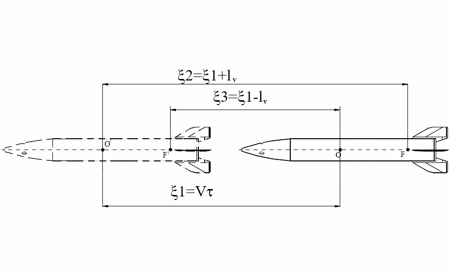
f (ξ) = \frac{R_{11} (ξ)}{σ^{2}} = lim X \to \infty \frac{1}{2 {X σ}^{2}} \int_{- X}^{X} u_{1} (x_{1}) u_{1} (x_{1} + ξ) {d x}_{1}

(8)

This function represents the correlation between velocity components along an axis, given in two points of that axis (Figure 1). On the basis of the hypothesis regarding isotropy:

Figure 1. Longitudinal correlation of velocity components.

f (ξ_{1}) = f (ξ_{2}) = f (ξ_{3}) = f (ξ)

(9)

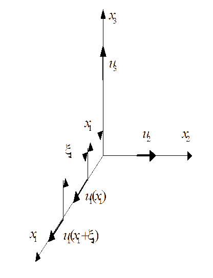
and:

f (ξ) = \frac{R_{11} (ξ_{1})}{σ^{2}} = lim X \to \infty \frac{1}{2 {X σ}^{2}} \int_{- X}^{X} u_{1} (x_{1}) u_{1} (x_{1} + ξ_{1}) {d x}_{1}

(10)

The other function, $g (ξ)$ , is the lateral correlation function given by the relation:

g (ξ) = \frac{R_{33} (ξ)}{σ^{2}} = lim X \to \infty \frac{1}{2 {X σ}^{2}} \int_{- X}^{X} u_{3} (x_{1}) u_{3} (x_{1} + ξ) {d x}_{1}

(11)

This function represents the correlation between the transversal velocity components with respect to an axis (Figure 2), defined at two points of that axis. Based on the hypothesis regarding isotropy:

Figure 2. Transversal correlation of velocity components.

u_{3} (x_{1}) u_{3} (x_{1} + ξ_{1}) > = < u_{2} (x_{1}) u_{2} (x_{1} + ξ_{1}) > = = < u_{3} (x_{2}) u_{3} (x_{2} + ξ_{2}) > = . . .

(12)

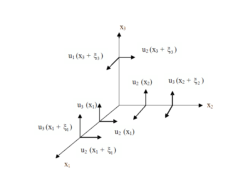
and:

g (ξ) = \frac{R_{33} (ξ_{1})}{σ^{2}} = lim X \to \infty \frac{1}{2 {X σ}^{2}} \int_{- X}^{X} u_{3} (x_{1}) u_{3} (x_{1} + ξ_{1}) {d x}_{1}

(13)

Uniform turbulence model

For the characteristic correlation functions, the following relations from [1] may be used:

f (ξ) = \frac{2^{2 / 3}}{Γ (1 / 3)} ζ^{1 / 3} K_{1 / 2} (ζ)

g (ξ) = f (ξ) - \frac{2^{- 1 / 3}}{Γ (1 / 3)} ζ^{4 / 3} K_{2 / 3} (ζ)

(14)

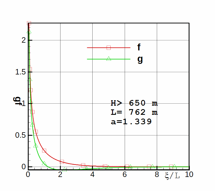
where: $ζ = \frac{ξ}{aL}$ , with $a = 1.339$ and L representing the characteristic length. $Γ$ is the second degree Euler function and $K_{υ}$ is the second degree Bessel modified function.

The characteristic functions defined by (14) are graphically represented in Figure 3.

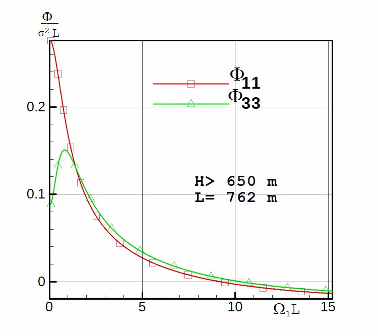
Figure 3. Characteristic correlation functions.

The Fourier transforms of the functions $f (ξ)$ and $g (ξ)$ are spectral one-dimensional functions related to longitudinal and lateral coordinates:

Φ_{11} (Ω_{1}) = \frac{σ^{2}}{π} \int_{0}^{\infty} f (ξ) e^{- i Ω_{1} ξ} d ξ

Φ_{33} (Ω_{1}) = \frac{σ^{2}}{π} \int_{0}^{\infty} g (ξ) e^{- i Ω_{1} ξ} d ξ

(15)

These functions are presented in Figure 4.

Figure 4. Characteristic spectral functions.

NOTE: For these spectral functions, through experimental measurements, several models have been established, among which, the most commonly used are the von Karman model.

Φ_{11} (Ω_{1}) = \frac{σ^{2} L}{π} \frac{1}{[1 + (aL Ω_{1})^{2}]^{5 / 6}}

Φ_{33} (Ω_{1}) = \frac{σ^{2} L}{2 π} \frac{1 + (8 / 3) (aL Ω_{1})^{2}}{[1 + (aL Ω_{1})^{2}]^{11 / 6}}

(16)

and the Dryden model:

Φ_{11} (Ω_{1}) = \frac{σ^{2} L}{π} \frac{1}{1 + (L Ω_{1})^{2}}

Φ_{33} (Ω_{1}) = \frac{σ^{2} L}{2 π} \frac{1 + 3 (L Ω_{1})^{2}}{[1 + (L Ω_{1})^{2}]^{2}}

(17)

The established experimental relations [1], are in good accordance with relations (15) and may be successfully used in the case of the study models with uniform turbulence. However, in the case of linear turbulence method, due to the necessity to define cross correlation functions which show the mutual dependence between velocity components, the characteristic functions defined by (14) will be used.

For the adopted models, both theoretical or experimental, we defined the characteristic length L and the turbulence intensity σ.

In case of altitudes over 650 m the boundary layer influence is diminished and the atmosphere may be considered, a unique value for the characteristic length L being recommended, both to longitudinal and lateral spectral functions. For the model considered, according to [1] L=762 m. The standard deviation is the same in all three directions, depending only on the turbulence intensity: σ=1.53 m/s is low turbulence; σ=3.05 m/s is mean turbulence; σ=6.4 m/s is height turbulence (storm).

The turbulence model obtained in this way is the simplest possible, being known as the uniform field model, in which only the linear components of velocity along the three axes, reduced in the gravity centre of the rocket, are considered: $u_{g}, v_{g}, w_{g}$ . Each component is considered uniform at each point of rocket’s surface.

The linear turbulence method

A higher-order approximation is the one of a linear field, with the turbulence velocities being considered as linear functions depending on position.

Authors of [1] and [2] developed in the case of airplanes linear turbulence models at four points. These models also allow calculation of rotation velocity components $p_{g}, q_{g}, r_{g}$ due to turbulence. Starting from the method proposed in [1], we developed for rockets a linear model of turbulence at two points, which allows deduction of the angular velocity of pitch and yaw motion. We briefly present this model in what follows.

In the linear turbulence case, due to the slender axi-symmetrical shape of the rocket, some gradients may be neglected. The influence of the remaining gradients may be considered as similar to supplementary rotation pitch and yaw velocities. To calculate these velocities we shall consider a model of the rocket in two points as shown in Figure 5, where point 0 represents the position of the mass centre and 1 represents the position of the configuration focal point.

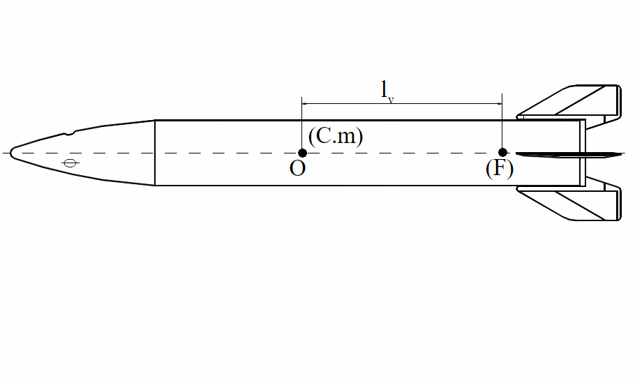
Figure 5. Model of the rocket in two points.

The length $l_{v}$ , called aerodynamic length, represents the distance from the mass centre to the focal point. Based on this model, the pitch and yaw velocities, equivalent to the velocity gradients, are:

q_{g} = \frac{1}{l_{v}} (w_{1} - w_{0})

;

r_{g} = \frac{1}{l_{v}} (v_{0} - v_{1})

(18)

to which there are added the linear velocities due translation for the uniform turbulence:

w_{g} = w_{0}

;

u_{g} = u_{0}

;

v_{g} = v_{0}

(19)

To calculate the velocities produced by turbulence, we expressed their correlation functions through the characteristic functions f and g, proceeding as in the case of uniform distribution, we calculated the spectral functions corresponding to the correlation functions and, from these, we found some possible forms of the translation and rotation velocities generated by turbulence.

For the case of the pitch turbulence velocity the following initial relation was used:

R_{qq} (τ) =< q_{g} (t) q_{g} (t + τ) >

(20)

which was expanded as:

R_{qq} (τ) = \frac{1}{(l_{v})^{2}} < (w_{1} - w_{0}) (w'_{1} - w'_{0}) > = \frac{1}{(l)^{2}} [< w_{1} w'_{1} > + < w_{0} w'_{0} > - w_{1} w'_{0} > - w_{0} w'_{1} >]

(26)

obtaining:

\frac{(l_{v})^{2}}{σ^{2}} R_{qq} (τ) = 2 g (ξ_{1}) - g (ξ_{2}) - g (ξ_{3})

(21)

where:

ξ_{1} = V τ

;

ξ_{2} = ξ_{1} + l_{v} ξ_{3} = ξ_{1} - l_{v}

To calculate the angular yaw velocity, a similar procedure was used:

R_{rr} (τ) = < r_{g} (t) r_{g} (t + τ) > = \frac{1}{(l_{v})^{2}} < (v_{0} - v_{1}) (v'_{0} - v'_{1}) > = \frac{1}{(l_{v})^{2}} [< v_{0} v'_{0} > + < v_{1} v'_{1} > - v_{1} v'_{0} > - v_{0} v'_{1} >]

(22)

from which we obtained:

R_{rr} (τ) = \frac{1}{(l_{v})^{2}} [2 R_{22} (V τ, 0,0) - R_{22} (V τ + l_{v} 0,0) - R_{22} (V τ - l_{v} 0,0)]

\frac{(l_{v})^{2}}{σ^{2}} R_{rr} (τ) = 2 g (ξ_{1}) - g (ξ_{2}) - g (ξ_{3})

(23)

From the previous relations and (13) for the characteristic functions f and g, the correlation functions for the rotation velocities were determined. The two rotation velocity components are equal, $R_{qq} = R_{rr}$ , due to axial symmetry. They are represented by a single correlation function in Figure 7.

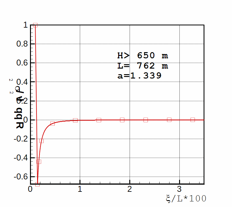
Figure 6. Correlation functions calculus schema.

Figure 7. Correlation function for rotation velocities.

Starting from the correlation function determined as above, by Fourier Transform we obtained the spectral function for the rotation velocity, represented in Figure 8.

To verify our calculus method, we compared the velocity components calculated with the linear turbulence field theory to those obtained using the uniform field theory. These proved to be identical.

Thus, for the longitudinal component we obtained:

R_{uu} (τ) =< u_{g} (t) u_{g} (t + τ) >=< u_{0} u'_{0} >= R_{11} (V τ, 0,0) = σ^{2} f (ξ_{1})

(24)

For the lateral component we obtained:

R_{vv} (τ) =< v_{g} (t) v_{g} (t + τ) >=< v_{0} v'_{0} >= R_{22} (V τ, 0,0) = σ^{2} g (ξ_{1})

(25)

R_{ww} (τ) =< w_{g} (t) w_{g} (t + τ) >=< w_{0} w'_{0} >= R_{33} (V τ, 0,0) = σ^{2} g (ξ_{1})

(26)

Relations (24), (25), and (26) show that for linear model we found the same characteristic f and g from Figure 3 and the spectral functions shown in Figure 4. This means that the translation velocities for the liner model are the same as those in the uniform model and for these we can use the theoretical relation (14) or the experimental relations (16) and (17).

Relations (23) for the angular velocities may only be used in the case of the theoretical model defined by the characteristic functions (14). In the case of axi-symmetric rockets, the only supplementary term specific to relations (23) is produced by the angular pitch/yaw velocities. If the aerodynamic length is comparable with respect to the characteristic length, the influence of this term is small and can be neglected. In the case of short rockets, like the anti-hail rocket, the term is important as we will see from the numerical comparison. On the other hand, for the rockets with an aerodynamic configuration more like an airplane, other coupling terms may be considered, so that the linear model is necessary.

Simulation of atmospheric turbulence

The simulation of an atmospheric turbulence is based on the Fourier Synthesis method. This method uses the spectral function modulus of the turbulence velocity to obtain the oscillation amplitude specific to a frequency bandwidth.

So, for the spectral functions values presented in Figure 4, by integration on small intervals, we determine the value of amplitude corresponding to a frequency bandwidth, which can be approximated with the frequency corresponding to the centre of the integrated domain. Moreover, for equal integrals, the values of the amplitudes will be the same, only the frequencies will be different. To complete the model, we associated to each frequency an initial arbitrary phase.

Using the notation $S_{φ}$ for the portion of the area obtained by integrating the modulus of a spectral function from Figure 4 and considering that the function has been represented only for the positive values of the variable $Ω_{1}$ , the amplitude has the value:

A = σ \sqrt{2 S_{φ}}

(27)

Two of the translation velocities generated by turbulence in a point $ξ$ are given by:

u_{g} (ξ) = A_{1} \sum_{i} sin (Ω_{1}^{i} ξ + φ_{1}^{i})

w_{g} (ξ) = A_{2} \sum_{i} sin (Ω_{2}^{i} ξ + φ_{2}^{i})

(28)

where the index ‘1’ was given to amplitude, pulsation and initial phase obtained from the modulus of the longitudinal spectral function, and the index ‘2’—given to the elements obtained from the modulus of the lateral spectral function. The third component of the velocity is the same as the second, excepting the initial phase:

v_{g} (ξ) = A_{2} \sum_{i} sin (Ω_{2}^{i} ξ + φ_{3}^{i})

(29)

Making the assumption that the rocket flies on a linear trajectory with a constant velocity V, the linear space variable may be expressed function of time by:

ξ = V τ

(30)

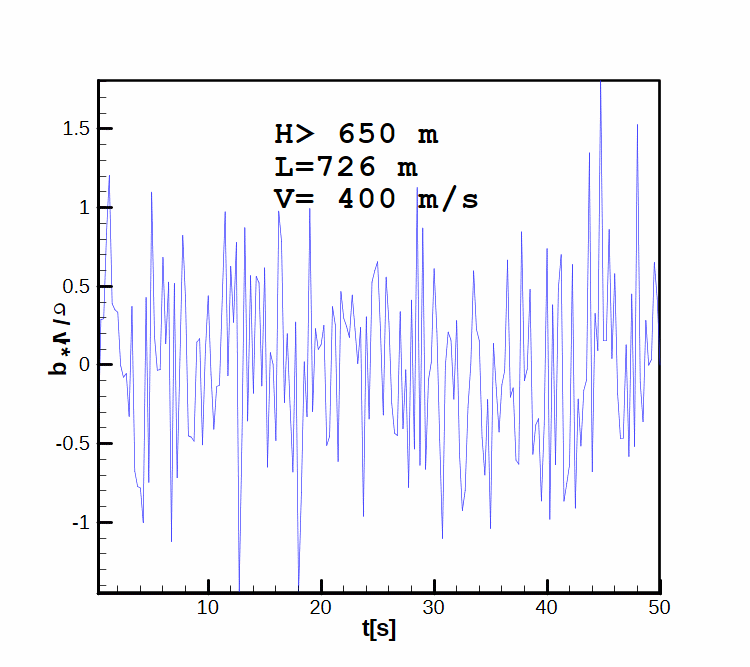
Consequently, the velocities originated by turbulence may be expressed as functions of time (Figure 9).

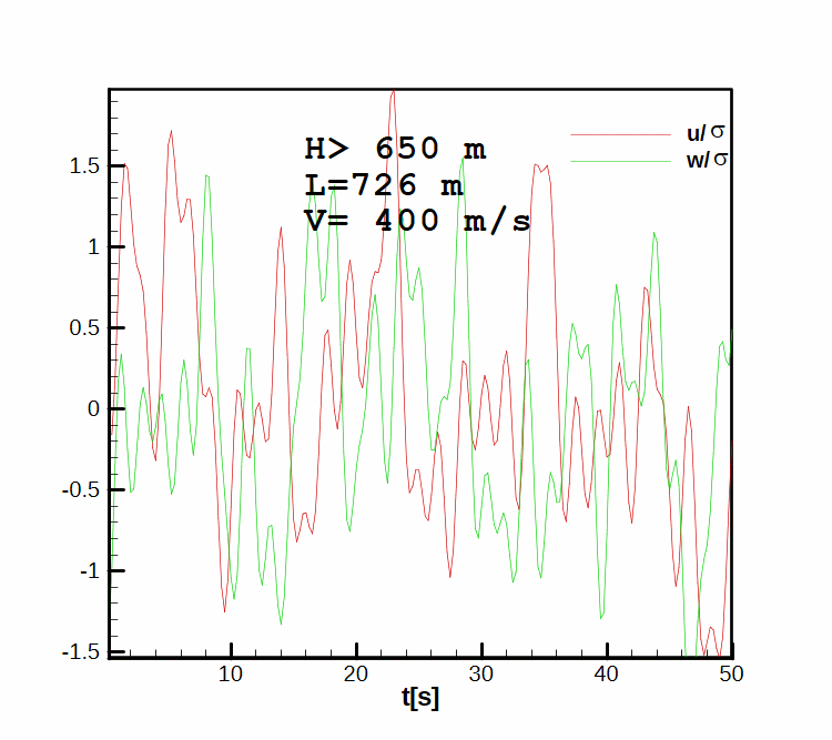
Figure 9. The axial ug and normal wg velocities produced by turbulence.

The modulus of the spectral functions presented in Figure 8 was used to find the angular velocities. By applying similar relations to (27) and (28) we obtained a form of the angular velocities originated by turbulence with respect to time. Noting that the spectral functions are equal, as it can be seen from Figure 8, the yaw and pitch velocities will be approximately equal $r_{g} \approx q_{g}$ , differing only by initial phases. In this case, in Figure 10, we presented only the pitch velocity function $q_{g}$ .

Figure 10. The pitch velocity produced by turbulence.

Anti-hailstone rocket trajectory

Some details regarding the procedure of building the simulation model [4] for the anti-hailstone rocket are presented in this section.

For the turbulent atmosphere we used the uniform and the linear turbulence model, in order to make a comparison. The initial values of the sinusoidal phases sums were obtained by generating random numbers, and the amplitude and frequency were determined starting from the spectral density functions from Figures 4 and 8, using the procedure described in the previous section. Because of the sequential initial random input of the phases, a fascicle of trajectories was obtained. The main stages of the trajectories were statistically analysed.

The results obtained by using the random number generator method are presented in the next tables.

In order to analyse trajectory parameters, we define six check points (stages):

Start point
End of rocket motor burn
Beginning of active substance spreading
Trajectory apex
End of active substance spreading
Impact point

In the next tables are presented numerical results for the nominal trajectory (without turbulence—Table 1), uniform model (Table 2) and liner model (Table 3). In Tables 2 and 3 there are two rows for each parameter: the first for average and the second for standard deviation values.

Table 1. Nominal trajectory parameter without turbulence =0.

Stage of flight	1	2	3	4	5	6
T [s]	0	9.5	14	26.1	36	58.
V [m/s]	40	625.4	400	209	179.5	206
γ [deg]	45	29.2	24.6	0.20	–28.0	–68.1
X [m]	0	2654	4669	7882	9691	12210
Y [m]	1	1788	2818	3677	3238	0
Z [m]	0	–0.5	–0.8	–0.75	–0.22	3.6

Table 2. Average and standard deviation trajectory parameters, low turbulence =1.53, uniform model.

Stage of flight	1	2	3	4	5	6
T [s]	0	9.5	14.	26.9	36.0	57.9
	0	0.0	0.0	0.1	0.0	0.59
V [m/s]	40	628.6	399.7	201.8	179.5	206.0
	0	0.3	0.7	0.9	1.0	0.73
γ [deg]	45	28.4	24.6	0.28	-28.0	-68.03
	0	0.24	0.6	0.19	0.5	0.47
X [m]	0	2672.2	4671.2	7907.9	9691.1	12207.7
	0	7.9	28.2	2.5	41.8	17.4
Y [m]	1	1755.5	2815.3	3980.1	3232.1	0
	0	11.17	42.8	30.8	96.6	0
Z [m]	0	–43.4	–2.2	33.7	–3.9	0.3
	0	15.05	49.3	64.4	100.76	130.7

Table 3. Average and standard deviation trajectory parameters, low turbulence=1.53, linear model.

Stage of flight	1	2	3	4	5	6
T [s]	0	9.5	14.	26.6	36.0	58.06
	0	0.0	0.0	0.1	0.0	0.97
V [m/s]	40	625.6	397.5	201.2	174.2	200.3
	0	0.3	0.8	1.9	2.5	1.6
γ [deg]	45	29.5	24.5	–1.	–28.4	–68.7
	0	0.54	0.9	0.39	0.4	1.24
X [m]	0	2644.3	4664.2	7846.0	9624.5	12018.0
	0	14.6	46.7	19.5	70.9	64.7
Y [m]	1	1801.0	2806.1	3862.1	3201.8	0
	0	17.7	73.1	41.2	159.6	0
Z [m]	0	1.1	37.2	–13.0	71.9	91.0
	0	4.9	29.3	20.4	62.3	77.3

In order to help analyse the numerical results, the main results are presented in a comparative form in Figures 11–16.

Figure 11. Velocity diagram average values—low turbulence.

Figure 12. Velocity diagram standard deviation values—low turbulence.

Figure 13. Climb angle diagram—average values, low turbulence.

Figure 14. Climb angle diagram—standard deviation values, low turbulence.

Figure 15. Trajectory diagram—average values, low turbulence.

Figure 16. Trajectory diagram—lateral coordinate, standard deviation values, low turbulence.

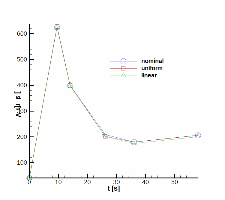
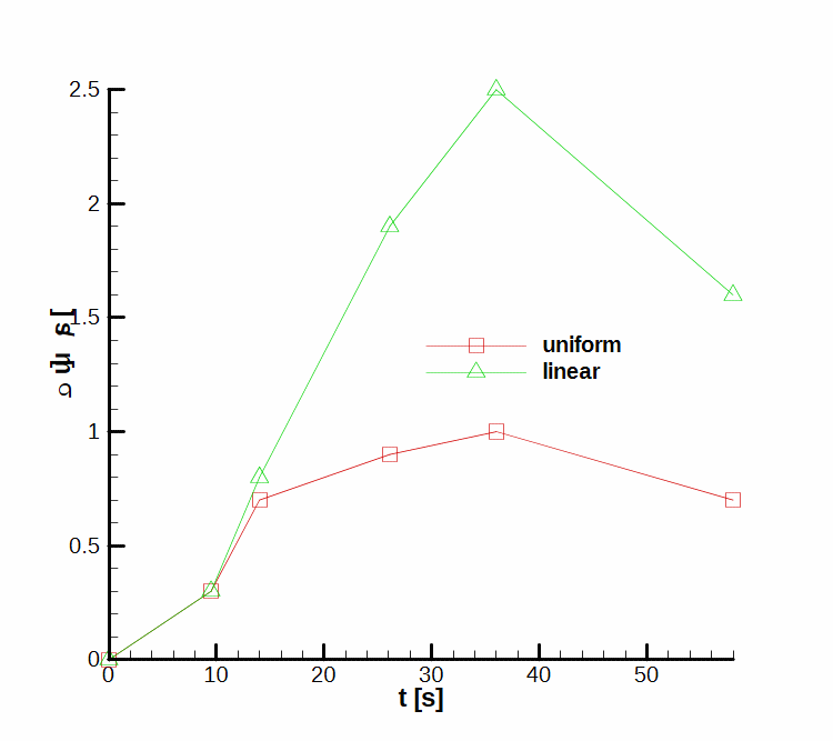
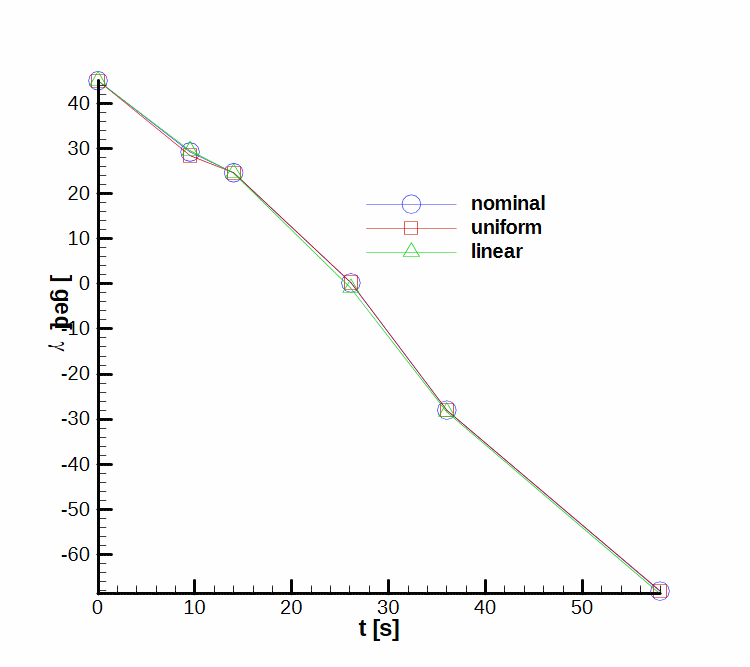
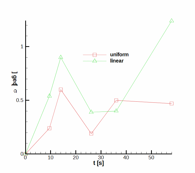
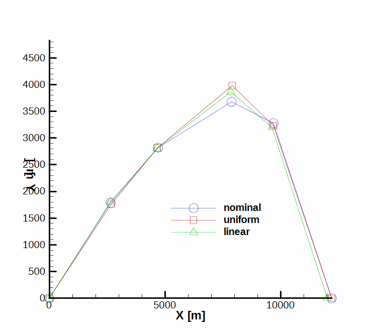
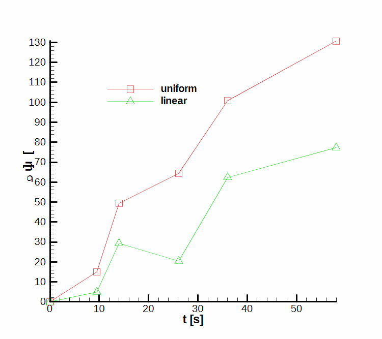
From the figures it can be observed that the average parameters from nominal trajectory, uniform model and linear model are relatively close. However, the dispersion parameters obtained with the uniform model and the linear model are not close, therefore the use of the linear model is justified.

Conclusions

Two turbulence models were presented in the paper. In the uniform turbulence model, only the translation velocities of the mass centre are considered. In the linear turbulence model, besides the linear velocities, the angular velocities of pitch and yaw with respect to mass centre are added.

In the case of axi-symmetric rockets, the term depending on angular velocities is the only which couples the equations. A further simplification could be made in the case of short rockets to which the distance between the mass centre and aerodynamic centre is much smaller than the characteristic length of the turbulent phenomena (L). In this situation, the coupling term due to rotations is small and may be neglected, so that the uniform turbulence model is an acceptable approximation.

In the case of long rockets, the coupling term contribution may be important. The same remark is valid for rocket plane-symmetric configuration. For both cases, supplementary coupling terms appear in the turbulence model, so the use of linear model is necessary.

Considering the linear turbulence model developed in our study, we have analysed in a simulation example the flight dynamics of a rocket, in which the influence of turbulence was evaluated in six stages of the flight. The contribution this study brings to the knowledge regarding unguided rocket flight is the technique used to modelling the turbulent atmosphere influence:

the two point model used to describe the linear turbulence,
the technique used to obtain the turbulence velocity, and
the comparison between linear and uniform turbulence models.

References

[1] B. Etkin, Dynamics of Atmospheric Flight, John Wiley & Sons, Inc., New York, 1972.

[2] T.V. Chelaru, Dinamica Zborului – Proiectarea avionului fără pilot , Ed. Printech, Bucureşti, aprilie 2003.

[3] T.V. Chelaru, Dezvoltare model statistic de calcul a împrăştierii traiectoriilor, din cadrul Proiectului RELANSIN “Ansamblu general mecanic pentru racheta antigrindină RAG 82”, contract 1322, etapa a II-a, iunie 2001.

[4] T.V.Chelaru, Dinamica Zborului—Racheta nedirijată, Ed. Printech Bucureşti, martie 2006.

Authors

Mircea Cernat was born in Romania, in 1957. He finished his PhD studies in 1996. He is the deputy director for science at Military Equipment and Technology Agency, Bucharest. Since 1987 he has worked in positions linked to education and research, having the title of professor at Military Technical Academy in Bucharest. He has managed or contributed as a member in research teams in several projects regarding weapon systems technology. His research topics are focused on applied mathematics to weapon systems and structural mechanics. Phone: +40-21-423.14.83, e-mail: mcernat@acttm.ro, fax +40-21-423.10.30.

Teodor-Viorel Chelaru was born in Romania, in 1956. He completed his Ph.D. studies in 1994. Since 1984 he has participated in a number of projects for guided and unguided missiles and UAV inside of the National Company for Military Technique. He is an Associate Professor at the POLITEHNICA University of Bucharest. His main research is focused on the dynamic flight and control of guided missiles.