Volume 10, Number 2, July 2007

Mathematical Calculation Model For Guidance Precision, Target Hit, And Target Kill Probabilities, In The Case Of Close Range-Homing Missiles

Teodor-Viorel I. Chelaru¹ and Mircea Cernat²

¹ University POLITEHNICA of Bucharest, Splaiul Independentei 313, Postal code 060032, Romania.
² Military Equipment and Technologies Research Agency, PO Box 51-16, 053070, Bucharest, Romania.

Abstract

This paper presents a random calculus model for guidance precision, and evaluation of target hit and target kill probabilities, in the case of close range-homing missiles. Due to their non-stationary character, the guidance equations have been integrated by canonical separation and the results have been analyzed by comparison for various tactical situations. Observations about the influence of various parameters on missile performance have been formulated. The novelty of the paper resides in application of the theoretical method, from random functions theory, to solve the technical problem of missile guided-flight modelling, for which we obtained some interesting and useful results.

Nomenclature

The main symbols utilized in this paper, according to [5], are listed below and described in Figure 1:

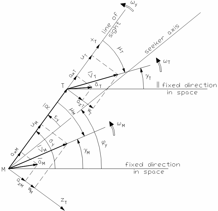
Figure 1. Two-points guidance kinematics.

$M$ : Missile;

$T$ : Target;

$MT$ : Line of sight (LOS);

$\bar{R}$ : Range;

$σ_{y}$ : Absolute angle of the LOS;

$γ_{M}$ : Missile climb angle;

$γ_{T}$ : Target climb angle;

$μ_{M}$ : Missile aspect angle;

$μ_{T}$ : Target aspect angle;

${\bar{V}}_{M}$ : Missile velocity;

$u_{M}$ : Missile velocity component along the LOS;

${\bar{V}}_{T}$ : Target velocity;

$u_{M}$ : Target velocity component along the LOS;

$ω_{y}$ : Angular velocity of LOS;

$ω_{M}$ : Missile angular rate of the velocity vector;

$ω_{T}$ : Target angular rate of the velocity vector;

$K$ : Proportional navigation constant;

$k$ : Modified navigation constant;

$t_{f}$ : Time to hit the target; and

$t_{go}$ : Time to go.

Introduction

The study of performance parameters is very important in the case of guided missile flight. The tactical performance parameters define the technical characteristics of a missile, for a set of given targets and launching conditions, setting the limits of its combat use.

According to [2], the tactical performance parameters include:

Dynamic launch zones (DLZ) for a given tactical situations, for a given type of missile integrated in a land, airborne, or naval firing system.
Guidance precision, error at the target, and target kill probability.

The problems related to launching zones and to target kill probability can be addressed either independently, as we have done in this paper, or inter-conditioned through complementary calculus models. In the latter case, we performed only the guidance precision calculation by means of random models built on the basis of the movement equations in their linear form.

Generally speaking, guidance precision determination is a difficult problem because it involves sophisticated mathematical calculus, based on knowledge of the field of random variable functions and equations. Further, in the case of homing missiles, these difficulties combine with the highly non-stationary character of the guidance kinematic equations, which require problem-solving approaches specific to this class of problems.

In this respect we stress that this is in contrast to the procedure for the evaluation of guidance precision for unguided rockets, which is mostly an experimental one and, in the case of missiles, is very expensive and extremely difficult to implement.

So, the only procedure we consider to be acceptable is that proposed through the model described in this paper (or something similar to it).

In the following, we analyse a random model used for determination of guidance precision and we propose a numerical solution for the equations we obtain; this solution is based on canonical development of the random variables.

Analytic model

To begin, we discuss an analytic model of this problem, as it is presented in papers [2,7].

Projecting the velocity and the acceleration along the LOS (see Figure 1) we obtain the following well-known scalar equations:

\dot{R} = u_{T} - u_{M}

; and

{\dot{σ}}_{y} R = w_{M} - w_{T}

, (1)

Respectively:

\ddot{R} - ω_{y}^{2} R = a_{xT} - a_{xM}

; and

{\dot{ω}}_{y} R + 2 \dot{R} ω_{y} = a_{zM} - a_{zT}

(2)

which represent kinematic equations in non-linear form for two-points guidance methods, including the proportional navigation (PN) case.

If the velocity and acceleration are expressed in terms of the components linked by velocity vectors for missile and target, the previous relations become:

\dot{R} = V_{T} cos μ_{T} - V_{M} cos μ_{M}

; and

{\dot{σ}}_{y} R = V_{M} sin μ_{M} - V_{T} sin μ_{T}

(3)

Respectively:

\ddot{R} - ω_{y}^{2} R = {\dot{V}}_{T} c o s μ_{T} - {\dot{V}}_{M} c o s μ_{M} + ω_{T} V_{T} s i n μ_{T} - ω_{M} V_{M} s i n μ_{M}

;

{\dot{ω}}_{y} R + 2 \dot{R} ω_{y} = ω_{T} V_{T} c o s μ_{T} - ω_{M} V_{M} c o s μ_{M} - {\dot{V}}_{T} s i n μ_{T} + {\dot{V}}_{M} s i n μ_{M}

(4)

Because of the variation in range R, (3) and (4) are non-stationary. They can be linearised around the basic direction of movement which is the collision trajectory [1] but they don’t abide Laplace or Fourier transformations through classic methods. After the linearisation of the acceleration kinematic equations (4) we obtain also a non-stationary movement equation:

R Δ {\dot{ω}}_{y} + 2 \dot{R} {Δ ω}_{y} + (\ddot{R} - ω_{y}^{2} R) {Δ σ}_{y} u_{T} {Δ ω}_{T} - u_{M} {Δ ω}_{M} + a_{xT} {Δ γ}_{T} - a_{xM} {Δ γ}_{M}

(5)

Adding the linear form of the PN law, where we consider the missile’s airframe with a first degree approximation:

H (s) = \frac{K}{1 + τ_{1} s}

and a random angular noise: $ε_{y}$ (see Figure 1):

{Δ ω}_{M} = \frac{K}{1 + τ_{1} s} ({Δ ω}_{y} + Δ {\dot{ε}}_{y})

(6)

we obtain the linear non-stationary guidance equation:

{R τ}_{1} Δ {\ddot{ω}}_{y} + (3 τ_{1} \dot{R} + R) Δ {\dot{ω}}_{y} + (2 \dot{R} + 2 τ_{1} \ddot{R} + u_{M} K) {Δ ω}_{y} = - u_{M} K Δ {\dot{ε}}_{y} + u_{T} (1 + τ_{1} s) {Δ ω}_{T} + + (1 + τ_{1} s) [a_{xT} {Δ γ}_{T} - a_{xM} {Δ γ}_{M} - (\ddot{R} - ω_{y}^{2} R) {Δ σ}_{y}]

(7)

To rewrite this equation in terms of miss distance, we write the angular velocity derivatives:

{Δ ω}_{y} = \frac{- \dot{R}}{R^{2}} Δ h

and

Δ {\dot{ω}}_{y} = \frac{- \dot{R}}{R^{2}} Δ \dot{h} - \frac{1}{R^{2}} (\ddot{R} - 2 \frac{{\dot{R}}^{2}}{R}) Δ h

Δ {\ddot{ω}}_{y} = \frac{- \dot{R}}{R^{2}} Δ \ddot{h} - \frac{2}{R^{2}} (\ddot{R} - 2 \frac{{\dot{R}}^{2}}{R}) Δ \dot{h} - \frac{6}{R^{3}} (\ddot{R} - 2 \frac{{\dot{R}}^{2}}{R}) Δ \dot{h}

(8)

where h is the instantaneous value of the miss distance. In this case, (7) becomes:

τ_{1} \frac{\dot{R}}{R} Δ \ddot{h} + \frac{\dot{R}}{R} [1 + τ_{1} \frac{- \dot{R}}{R} (1 - 2 \frac{\ddot{R} R}{{\dot{R}}^{2}})] Δ \dot{h} + \frac{u_{M} K}{R} \frac{\dot{R}}{R} [1 - \frac{\ddot{R}}{u_{M} K} (τ_{1} + \frac{R}{- \dot{R}})] Δ h = u_{M} K Δ {\dot{ε}}_{y} - u_{T} (τ_{1} s + 1) {Δ ω}_{T} + + (τ_{1} s + 1) [a_{xM} {Δ γ}_{M} - a_{xT} {Δ γ}_{T} + (\ddot{R} - σ_{y}^{2} R) {Δ σ}_{y}]

(9)

Considering the link between the classical navigation constant K and the modified one [1] k:

u_{M} K = - \dot{R} k

(10)

from (9) we obtain the equation indicated in [2]:

τ_{1} Δ \ddot{h} + [1 + τ_{1} \frac{- \dot{R}}{R} (1 - 2 \frac{\ddot{R} R}{{\dot{R}}^{2}})] Δ \dot{h} - \frac{- \dot{R} k}{R} [1 - \frac{\ddot{R}}{- \dot{R} k} (τ_{1} + \frac{R}{- \dot{R}})] Δ h = k R Δ {\dot{ε}}_{y} + u_{T} \frac{R}{- \dot{R}} (τ_{1} s + 1) {Δ ω}_{T} - \frac{R}{- \dot{R}} (τ_{1} s + 1) [a_{xM} {Δ γ}_{M} - a_{xT} {Δ γ}_{T} + (\ddot{R} - σ_{y}^{2} R) {Δ σ}_{y}]

(11)

Furthermore, considering the notations:

a_{1} = \frac{- \dot{R} k}{{R τ}_{1}} [1 - \frac{\ddot{R}}{- \dot{R} k} (τ_{1} + \frac{R}{- \dot{R}})]

;

a_{2} = \frac{1}{τ_{1}} [1 + τ_{1} \frac{- \dot{R}}{R} (1 - 2 \frac{\ddot{R} R}{{\dot{R}}^{2}})]

;

b_{1} = - \frac{kR}{τ_{1}}

;

b_{2} = \frac{R}{- \dot{R} τ_{1}}

;

b_{3} = \frac{R}{- \dot{R} τ_{1}} (τ_{1} s + 1) [a_{xM} {Δ γ}_{M} - a_{xT} {Δ γ}_{T} + (\ddot{R} - σ_{y}^{2} R) {Δ σ}_{y}]

;

{Δ f}_{T} = u_{T} (τ_{1} s + 1) {Δ ω}_{T}

(12)

as well as the input $X = {Δ ε}_{y}$ and output $Y = Δ h$ , (11) becomes:

\ddot{Y} + a_{2} \dot{Y} + a_{1} Y = b_{1} \dot{X} + b_{2} {Δ f}_{T} + b_{3}

(13)

Where X, Y are random variables, and the a_i, b_i coefficients are time-dependent. Furthermore, writing:

Y_{1} = Y

and

Y_{2} = \dot{Y} - b_{1} X

(14)

(13) can be written in the form of a system with two first-order differential equations:

{\dot{Y}}_{1} = Y_{2} + b_{1} X

{\dot{Y}}_{2} = - a_{2} Y_{2} - a_{1} Y_{1} - a_{2} b_{1} X + b_{2} {Δ f}_{T} + b_{3}

(15)

If the input value is centred with $M (X) = 0$ , the system (15) can be rewritten in terms of the average functions:

{\dot{m}}_{y 1} (t) = m_{y 2}

{\dot{m}}_{y 2} (t) = - a_{2} m_{y 2} (t) - a_{1} m_{y 1} (t) + b_{2} {Δ f}_{T} + b_{3}

(16)

where:

m_{y 1} (t) = M_{}

and

m_{y 2} (t) = M_{}

(17)

The angular error at launch can be taken into account by the initial conditions imposed on (16):

m_{y 10} = {Δ h}_{0} = u_{M} t_{f} {Δ μ}_{M}

m_{y 20} = 0

(18)

To analyze the random component of the system in the equations (15), the relations (16) can be subtracted from the relations (15), and written in terms of centred random values:

\frac{d \overset{\circ}{Y_{1}}}{d t} = \overset{\circ}{Y_{2}} + b_{1} \overset{\circ}{X}

\frac{d {\overset{\circ}{Y}}_{2}}{d t} = - a_{2} \overset{\circ}{Y_{2}} - a_{1} \overset{\circ}{Y_{1}} - a_{2} b_{1} \overset{\circ}{X}

(19)

In [2] the average equations (16) and the dispersion equations (19) are solved by analytical means, but the solutions are very complicated. Hereinafter we propose a numerical solution.

Numerical method

In the following, we present a numerical method based on canonical separation of the random variables to solve this class of problems, which can be implemented easily in calculus software. The method consists of integrating the equations (19) using the canonical separation of random functions, according to the theory presented in [4].

This method allows the output signal dispersion to be obtained from the input signal dispersion for any kind of differential linear non-stationary equations using a decomposition of input signal in a number of pulsation domains (PD) and integrate differential equation system for each of them. The method is approximate, because the number of PD is limited. Theoretically, if we use an infinite number of PD we can obtain the exact solutions. To evaluate the accuracy of the method we first analyze a simple case, to provide a test case, with known analytical solutions.

Therefore, we choose, as example, the well-known linear stationary equation with constant coefficients:

τ_{1} \dot{y} + y = x

(20)

After the Laplace transformation, the equation can be written as a transfer function:

y = \frac{1}{τ_{1} s + 1} x

(21)

For a input random variable X, similar to ‘white noise’, centred around zero, at the output we will obtain a random signal Y also centred in zero. The analytical link between spectral densities of the signals is given by:

S_{y} = {| \frac{1}{τ_{1} i ω + 1} |}^{2} S_{x} = \frac{1}{τ_{1}^{2} ω^{2} + 1} S_{x}

(22)

The dispersion of the output signal can be obtained through integration of the spectral density with respect to the pulsation ω:

D_{y} = 2 \int S_{y} d ω = lim_{ω \to \infty} \frac{2 S_{x}}{τ_{1}} arctan τω = \frac{{π S}_{x}}{τ_{1}}

(23)

where the input signal doesn’t depend on pulsation.

As a numerical example: with time constant $τ_{1} = 0.5 [s]$ , input signal $S_{x} = 0.00394 [s]$ , and dispersion $D_{x} = 1$ for a maximum pulsation of $ω_{max} = 127 [1 / s]$ —using the analytical relation (23), $D_{yA} = 0.02468$ .

For the calculus example we observed that the PD for the spectral density of the output signal is limited, with the transfer function (21) working as a low-pass filter removing the high frequencies. In this application, therefore, we could approximate the spectral density of the input signal with a rectangle which contains PD in which the output spectral density has values (see Figure 2).

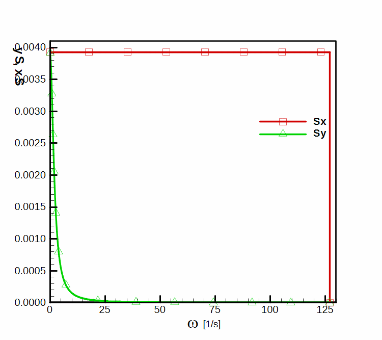
Figure 2. Spectral density for input and output signal.

Hereafter we apply the canonical separation method following [4] in which it is shown that for a non-stationary function $X$ it can be used a canonical separation:

$X (t) = m_{x} (t) + \overset{\circ}{X (t)} = m_{x} (t) + \sum_{k = 1}^{n} V_{k} ϕ_{k}$

where: $\overset{\circ}{X}$ is centred non-stationary function; $m_{x}$ is average function; $V_{k}$ are random quantities; and $ϕ_{k}$ are coordinate determinist functions. This work, [4], also shows the link between coordinate functions of the input-separated signal and the output-separated signal. This link allows building the spectral density and dispersion of the output signal using the spectral density of the input signal.

Supposing that the input signal is stationary (that is, the coordinate functions have a particular form $ϕ_{k} (t) = e^{{i ω}_{k} t}$ ) and centred, we can use the following decomposition:

\overset{\circ}{X} = \sum_{k = - n}^{n} W_{k} e^{{i ω}_{k} t}

, (24)

where $W_{k}$ it is complex random centred quantity with the dispersion $D_{k} = 2 D_{K}^{} = 2 D [W_{k}]$ obtained from the spectral density for the input signal $S_{x} (ω_{k}) = 2 S_{x}^{} (ω_{k})$ corresponding a pulsation band ${Δ ω}_{k}$ centred in pulsation $ω_{k}$ . Because the input signal is even, we can write:

D_{x} = \sum_{k = - n}^{n} D_{k}^{} = \sum_{k = 1}^{n} D_{k}

(25)

If the coordinate functions for the input signal are $ϕ_{k} (t) = e^{{j ω}_{k} t}$ and the coordinate functions for the output signal are $ψ_{k}$ , the dispersion for the output signal can be obtained with the relation:

D_{Y} (t) = 2 \sum_{k = 1}^{n} {D_{k} | ψ_{k} (t) |}^{2}

(26)

where the coordinate functions of the output signal can be obtained from the coordinate functions of the input signal through (20). We can build an equation system, containing an equation for each pulsation $ω_{k}$ :

{\dot{ψ}}_{k} (t) = - ψ_{k} (t) / τ + ϕ_{k} (t) / τ

(27)

where $k = 1 . . . n$ .

Because the functions $ϕ_{k}$ and $ψ_{k}$ are complex, the solution of the system (27) can be obtained by separating the imaginary part from real part:

{\dot{y}}_{1_{k}} (t) = - y_{1 k} (t) / τ + cos (ω_{k} t) / τ

{\dot{y}}_{2_{k}} (t) = - y_{2 k} (t) / τ + sin (ω_{k} t) / τ

(28)

where: $y_{1 k} = Re ψ_{k}$ ; $y_{2 k} = Im ψ_{k}$ , and $k = 1 . . . n$ .

Together with the system solution we obtain the square of the coordinate function corresponding to the pulsation $ω_{k}$ : $ψ_{k}^{2} = y_{1 k}^{2} + y_{2 k}^{2}$ , and also the dispersion corresponding to the pulsation band ${Δ ω}_{k}$ : $D_{k} = S_{x} {Δ ω}_{k}$ . Using relation (26) until maximum pulsation $ω_{max} = 127$ , for a pulsation number $n = 500$ and time $t_{max} = 5$ , we obtain the output signal dispersion, which for numerical application has the value $D_{yN} = 0.02443$ . For this application we directly evaluated the relative error between analytical result and numerical result:

Δ % = \frac{D_{yA} - D_{yN}}{D_{yA}} 100 = \frac{π - 2 \cdot atan (τ_{1} ω_{max})}{π} 100

(29)

which, for our application and selected values is: $Δ % ≃ 1 %$ .

From (29) we observe a numerical dependence between the maximum pulsation $ω_{max}$ , the time constant $τ_{1}$ and the relative error $Δ$ , which is valid for any system based on the delay function given by the time constant $τ_{1}$ , such as in the guidance system equation analysed in our work. In this case, for a value given to the time constant $τ_{1}$ we can impose a relative error $Δ$ which allows the choice of a value for maximum pulsation $ω_{max}$ . This is one of the advantages of this method: the possibility to estimate the calculus error choosing a reasonable value for maximum pulsation, which doesn’t involve huge calculus resources.

To solve (19) more easily we considered a non-stationary movement with constant velocity (without longitudinal acceleration). In this case, the relations (12) have a simplified form:

a_{1} (t) = \frac{k}{t_{go} τ_{1}}

;

a_{2} (t) = \frac{t_{go} + τ_{1}}{t_{go} τ_{1}}

b_{1} (t) = k {\tilde{u}}_{T} \frac{t_{go}}{τ_{1}}

(30)

b_{2} (t) = \frac{t_{go}}{τ_{1}}

;

b_{3} = 0

;

{Δ f}_{T} = u_{T} {Δ ω}_{T}

where: $t_{go} = t_{f} - t$ is time to go.

The simplification is not compulsory and does not affect the general character of the proposed method. Additionally, this method enabled us to solve the case when the missile airframe is described by a higher-order system, in a different way than the analytical method proposed in [2].

The deterministic system (16) with the given conditions (18) can be solved easily by numerical integration. To solve the non-stationary random system (19), we assume that the input value $\overset{\circ}{X}$ is stationary centred, and can be obtained by a canonical separation of the type:

\overset{\circ}{X} = \sum_{k = - n}^{n} W_{k} e^{{j ω}_{k} t}

(31)

where the oscillation amplitudes $W_{k}$ are random stationary centred complex values, and their dispersion $D_{k} = 2 D_{K}^{} = 2 D [W_{k}]$ can be obtained from the spectral density function of the input value $S_{x} (ω_{k}) = 2 S_{x}^{} (ω_{k})$ , corresponding to a pulsation band centred in $ω_{k}$ . As the input function is even, we can write:

D_{x} = \sum_{k = - n}^{n} D_{k}^{} = \sum_{k = 1}^{n} D_{k}

(32)

If we have the input value coordinate functions $ϕ_{k} (t) = e^{{j ω}_{k} t}$ and the complex coordinate functions of the output values: $ψ_{k}$ for $\overset{\circ}{Y_{1}}$ and $θ_{k}$ for $\overset{\circ}{Y_{2}}$ , the output values dispersions can be determined with the relations:

D_{Y 1} (t) = 2 \sum_{k = 1}^{n} {D_{k} | ψ_{k} (t) |}^{2}

D_{Y 2} (t) = 2 \sum_{k = 1}^{n} {D_{k} | θ_{k} (t) |}^{2}

(33)

where the coordinate functions of the output values corresponding to the pulsation k can be obtained by solving the system:

{\dot{ψ}}_{k} (t) = θ_{k} (t) + b_{1} ϕ_{k}

{\dot{θ}}_{k} (t) = - a_{2} θ_{k} (t) - a_{1} ψ_{k} (t) - a_{2} b_{1} ϕ_{k}

(34)

where $k = 1 . . . n$

Since $ϕ_{k}$ , $ψ_{k}$ , and $θ_{k}$ are complex functions, the equations (34) will be solved by separation of the real and the imaginary parts:

{\dot{y}}_{1 k} (t) = y_{3 k} (t) + b_{1} cos (ω_{k} t)

{\dot{y}}_{2 k} (t) = y_{4 k} (t) + b_{1} sin (ω_{k} t)

{\dot{y}}_{3 k} (t) = - a_{2} y_{3 k} (t) - a_{1} y_{1 k} (t) - a_{2} b_{1} cos (ω_{k} t)

{\dot{y}}_{4 k} (t) = - a_{2} y_{4 k} (t) - a_{1} y_{2 k} (t) - a_{2} b_{1} sin (ω_{k} t)

(35)

with $k = 1 . . . n$ , $y_{1 k} = Re ψ_{k}$ , $y_{2 k} = Im ψ_{k}$ , $y_{3 k} = Re θ_{k}$ , and $y_{4 k} = Im θ_{k}$ .

Thus we obtain a system containing four differential equations for each pulsation considered, which can be solved by numerical methods. For the equations (35) the initial conditions are considered zero.

NOTE: If the system input function $X$ is random (‘white noise’-like), the canonical separation involves a high number of terms situated on an infinite pulsation band. But considering the fact that the system works like a low-pass filter, the dispersion of the spectral development of the output value have significant values only up to a limited frequency, and that frequency can be also used as a limit for the spectral development of the input value.

Application on a calculation model

As an example, we consider a calculation model for a surface-to-air missile. Within this model we consider:

$u_{M} = 527 m/s$ —missile velocity along LOS;

$D_{0} = 50 m$ —the “blinding” distance;

$τ_{1} = 0.55 [s]$ —the time constant of the missile airframe;

K—the navigation constant:

$K = 2.0$ —‘receding ’ target;

$K = 2.88$ —‘approaching’ target;

$t_{f} = 11 s$ —maximum time of flight; and

$σ_{x} = 0.5 °$ —standard deviation of the input value.

The diagrams have been obtained by numerical integration of the average equations (16) with the initial conditions (18), considering ${Δ μ}_{M} = 2 °$ and zero initial conditions for the equations (19). The random input value X can be defined on the basis of the command system signal-to-noise-ratio, or by analysing the command surfaces oscillation in the absence of the guidance signal. The final values of the average miss distance obtained from equation (16) are presented in Figures 3 and 4. Figure 3 presents the average miss distance in the case of a non-manoeuvrable target, for various target velocities. The positive components of the target velocity along the LOS correspond to the receding target, and the negative ones, to the approaching target. All the samples show that, after the initial regime has ended, in the case of a non-manoeuvrable target, the average miss distance approaches zero.

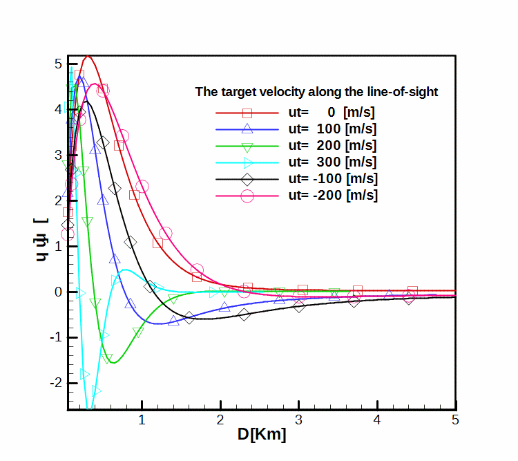
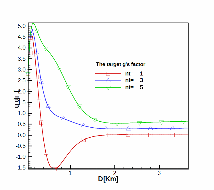
Figure 3. Average miss distance as a function of launch distance, for a non-manoeuvrable target.

Figure 4. Average miss distance as a function of launch distance, for a manoeuvrable target.

Figure 4 also analyses the average miss distance, but this time for a manoeuvrable target. All the curves in this diagram have been calculated considering the target velocity along the LOS: $u_{T} = 200 m/s$ . Analysing the diagram, we see that in the case of manoeuvrable target, the final value of the average miss distance is not zero, no matter how long the flight may be.

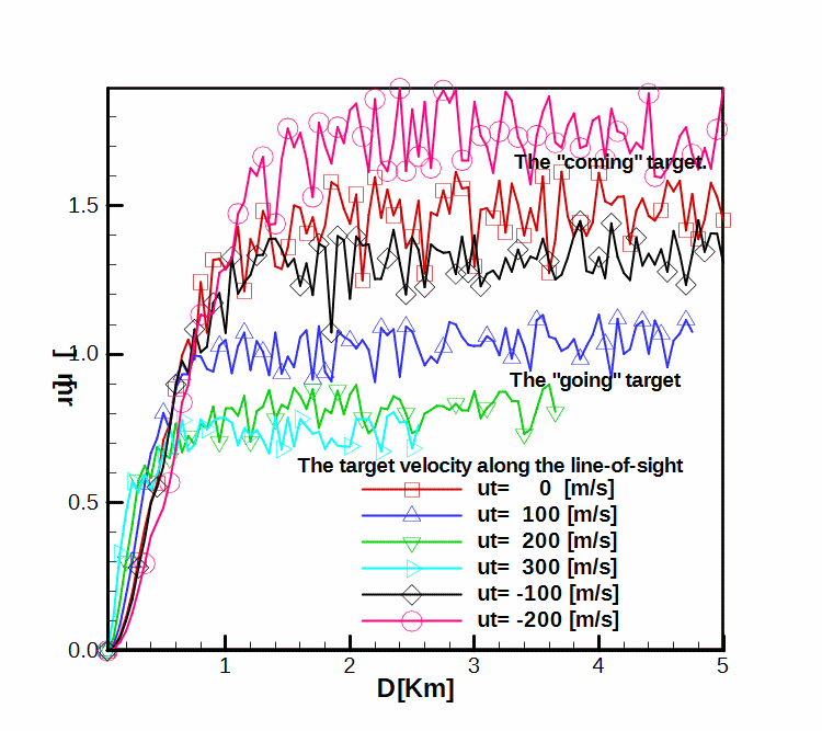
From the coordinates equations (35), for study model case considered, we have obtained the total dispersion circle radius ( $r = 4 A_{p}$ ) variation depending on the launch distance.

The results are shown in Figure 5. Analysing the diagram, we note that the results for approaching target are separated from the receding target results, this separation being caused by different values of the command system amplification in the two cases considered. The diagram curves are equivalent to those from Figure 3, corresponding to the various target velocities along the LOS.

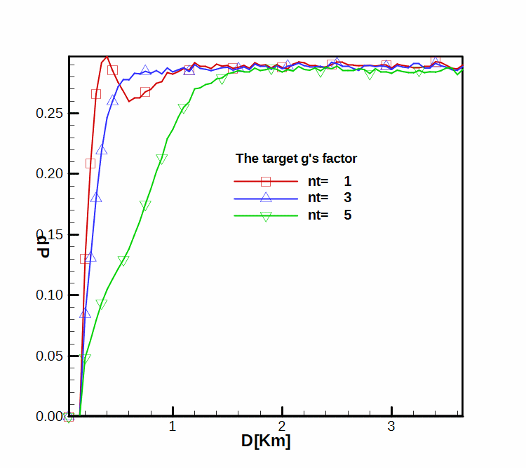
Figure 5. Total dispersion radius as a function of launch distance, for a non-manoeuvrable target.

In the following, knowing the standard deviation of the dispersion at the target and assuming a target with an equivalent surface of 9 m² and a proximity fuze detonation radius of 2 m, we found the single-shot hit probability: $w$ which is approaching unity for the considered application. Finally, applying the relation:

P_{d} = 1 - (1 - {wz}_{1} z_{2})^{n}

(36)

the target kill probability has been determined, considering for this application: $z_{1} = 0.6$ —the reliability $z_{2} = 0.55$ —the single-shot target kill probability (the effect at the target); n=1—the number of missiles. The results obtained are presented in Figure 6.

Figure 6. Target kill probability as a function of launch distance, in the case of a manoeuvrable target.

Conclusions

The results obtained show that the numerical integration method, applied to the guidance random equations with the random variables, gives good results if a high number of frequencies is selected. Although the solution appears to be complicated, leading to a high number of equations (four times the number of frequencies), it still is, due to its symmetry and generality character, a convenient method for solving these categories of problems, the majority of them having no analytic solutions. In terms of results obtained with the considered calculus model, it can be said that the average miss distance is not influenced by target velocity, if the target flies with a constant velocity on a straight flight path. It has also been concluded that in the case of a target which is not in the proximity of the launching point, the initial launching error, if kept within certain limits, does not affect the final value of the miss distance. On the other hand, target manoeuvres, even if they are constant, can lead to an increased average miss distance. The dispersion at the target is influenced, first of all, in a direct manner by the amplification coefficient, and high values of the navigation constant can lead to a significant increase of the equal probability circle (CEP).

The novel aspect of the paper resides in its technical purpose, that of finding solutions to a real problem, using an adequate model from random function class. Even if the model to determine the solution were to be subject to improvements, the results obtained here are technically acceptable and useful.

References

[1] R.Carpantier, Guidance des avions et des missiles aerodynamiques. , Tom I,II,III, lit. ENSAE - 1989.

[2] I.E. Kazakov and A.F. Mişakov, Aviaţionnîe upravliaemîe raketî -(„Airborne Guided Rockets”, in Russian), Ed. VVIA "N.E. Jukovski", 1985.

[3] N.T. Kuzovkov, Sistemî stabilizaţii letatelnîh appararov, balisticeschih i zenitnîh raket, („Stabilization Systems for Aircraft, Ballistic and Surface-to-air Missiles”, in Russian) Ed. Vîsşaia Şkola , Moskva, 1976.

[4] E.S. Venţeli, Teoria veroiatnostei—(„Probabilities Theory”, in Russian), Ed. Nauka, Moskva, 1964.

[5] STP M 40455-99—Sistemul rachetă dirijată („The Guided Rocket System”, in Romanian), Bucureşti, 1999.

[6] V.Chelaru and L.Dobre, , Studiu comparativ al ecuaţiei autodirijării utilizînd modelul dinamic şi cinematic al rachetei – (Comparison Study of the Self-guidance Equation using the Missile’s Dynamical & Kinematical Model, in Romanian), Revista Tehnica Militară, Nr. 1 -1993, Bucureşti, iunie - 1993

[7] T.V.Chelaru, Dinamica zborului—Racheta dirijată—Ed. 2 revizuită şi adăugită, Editura Printech, Bucureşti, 2004.

Authors

Teodor-Viorel Chelaru completed PhD studies in 1994 with the thesis "The studies of the dynamic flight for the guided missiles". Since 1984 he has participated on a various number of projects for guided and unguided missiles and UAV inside of the National Company for Military Technique. He is also an Associate Professor at the POLITEHNICA University of Bucharest. His main research is focused in the dynamic flight and control of guided missiles and UAV. Phone: +(40)0723214423,e-mail: t.v.chelaru@rom-arm.ro.

Mircea Cernat completed PhD studies in 1996 with the thesis entitled “Study of the solid propellant burning chambers under dynamic loading”. He is the deputy director for science at Military Equipment and Technology Agency, Bucharest. Since 1987 he worked in positions linked to education and research, having the title of professor at Military Technical Academy in Bucharest. His research topics are focused on applied mathematics to weapon systems and structural mechanics. Phone: +40-21-423.14.83, e-mail: mcernat@acttm.ro.

Figure 5. Total dispersion radius as a function of launch distance, for a non-manoeuvrable target.

Figure 6. Target kill probability as a function of launch distance, in the case of a manoeuvrable target.