
Volume 10, Number 1, March 2007
An Introduction To Electro-Explosive Hazard Assessment
- 1 Antuition Enterprises, 4 Kipling Street, Moonee Ponds, Victoria, 3039, Australia.
Abstract
The electromagnetic environment (EME) in both civilian and defence arenas continues to grow in complexity and intensity. At the same time complex electronic and electric control of a multitude of systems including those involving explosive ordnance (EO) is becoming commonplace. Paralleling this growth is, or should be, a heightened awareness of the EME and its effects including those from electromagnetic radiation hazards to ordnance, personnel, fuel, and electronic devices. Duty of care requires that the risks arising from these interactions be maintained at acceptable levels. This paper is intended to provide the novice, with minimal background in electromagnetics and explosives, some insight into the nature of electro-explosive hazards (EEH). While hazards arise from a number of electromagnetic phenomena, because of space limitations, this paper is limited to those associated with radio and radar transmission equipment, and the methodologies that can be used to estimate and manage such hazards.
Introduction
The electromagnetic environment (EME) in both civilian and defence arenas continues to grow in complexity and intensity. At the same time complex electronic and electric control of a multitude of systems including those involving explosive ordnance (EO) is becoming commonplace. Paralleling this growth is, or should be, a heightened awareness of the EME and its effects including those from electromagnetic radiation hazards to ordnance, personnel, fuel, and electronic devices. Duty of care requires that the risks arising from these interactions be maintained at acceptable levels. This paper is intended to provide the novice, with minimal background in electromagnetics and explosives, some insight into the nature of electro-explosive hazards (EEH). While hazards arise from a number of electromagnetic phenomena, because of space limitations, this paper is limited to those associated with radio and radar transmission equipment, and the methodologies that can be used to estimate and manage such hazards. It also addresses some cherished misconceptions.
Electro-explosive hazards (EEH)
EEH refers to the risk of an undesirable response of electrically initiated or controlled EO to the EME. This may range from uncommanded initiation of the EO, to degraded performance or failure to operate when required. The risk associated with such hazards needs to be managed over the whole life cycle of the EO, which includes storage, transport, handling and loading, presence in a weapon system, maintenance and disposal. An EEH assessment may need to address EO in any or all of these configurations.
The susceptibility of an item of EO in any particular configuration, is a function of three main factors:
- The EO and its weapon system. This involves not only the initiating component—the electro-explosive device (EED)—its characteristics and response, but the design of the weapon system and its platform;
- The characteristics of the EME. This involves the various electromagnetic phenomena to which the EO may be subject during its life; and
- The coupling methods that may exist between the two. This involves the mechanisms by which unwanted energy from the environment may couple directly or indirectly into the EED.
There exist a number of different assessment methodologies, which have been developed to address EEH, and translation of data between different methodologies is not always easy. In P236.94 [1], the Australian Ordnance Council (now the Director of Ordnance Safety (DOS)) endorsed the assessment methodology contained in P101 [2], now at issue 2. This methodology has been developed by UK DOD over many years and provides a rigorous and flexible approach to assessment. The US Navy uses the HERO methodology espoused in MIL-HDK-240 [3]. While both address the same issues, there are significant differences between the methodologies and the assumptions that are made. Assessments against P101 and HERO are not directly comparable and great care needs to be taken when extrapolating between the two. The term HERO should never be used as a generic term for EEH.
Electro-explosive systems and EEDs
The EED is a key component of any electro-explosive system. It provides the mechanism for release of chemical energy in response to an electrical stimulus, thus providing the trigger for initiation of the remainder of the explosive sequence. EEDs are found in a wide range of systems including warheads, rocket motors, gas generators, flares, smoke grenades, thermal batteries, cable cutters, and explosive bolts. While EEDs offer the advantages of simple control, reliability, low power requirements, and rapid response time, they are not able to distinguish between an intentional firing signal, and an inadvertent one. Without adequate design and handling procedures, energy from the EME can initiate the EED directly as a result of currents induced in EED firing circuits, or indirectly as a result of uncommanded operation of firing circuit switches or control systems. The ramifications are that the whole design of EED firing circuits, which may include electronic devices, microprocessors, and associated software, can have a significant bearing on the susceptibility. There are a number of different types of EED, some of which are described in this section.
The most common is the bridgewire (BW) EED. This consists of a thin filament of resistance wire, embedded in a temperature-sensitive explosive. Passage of electric current through the bridgewire will heat adjacent explosive, and if the temperature rise is sufficient, will lead to initiation. A related EED is called the film-bridge (FB) EED, which uses a conductive metallic film in lieu of the bridgewire.
Figure 1 shows a typical uncased bridgewire—an ‘E’-type fusehead. The firing current is introduced through the firing leads at the top left. The EED is designed to initiate in response to current to passing in one firing lead and out the other, and this is called the differential mode. The BW EED in Figure 2 is enclosed in a grounded metal case, and is also designed to initiate in the differential mode. However, even if there is no current passing through the bridgewire, if the voltage on both leads is sufficiently high the EED can be initiated by an electrical discharge through the explosive from the bridgewire to the case. This undesirable initiation mode is called the common mode, and generally arises from electrostatic discharge or when subject to very high electromagnetic fields.
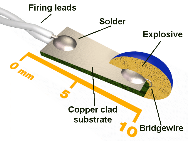
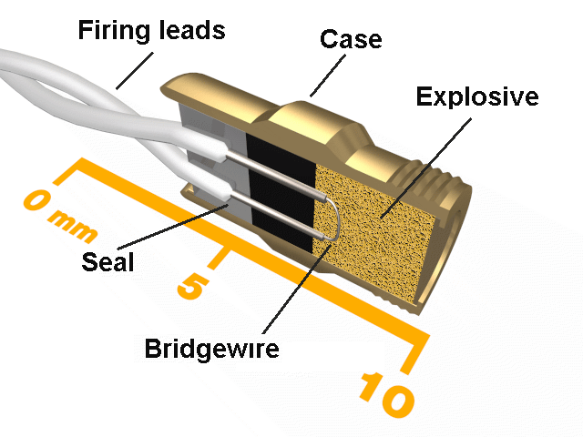
Figure 3 shows a conductive-composition (CC) EED. This contains an explosive mix intentionally made conductive by inclusion of an electrically conductive compound such as graphite. The firing current passes from the centre pole-piece to the outer case through microscopic conductive paths within the explosive mix. This leads to local hot-spots on a microscopic scale, and subsequent initiation.
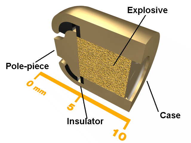
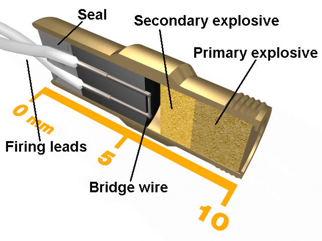
Figure 4 shows an exploding bridgewire (EBW) EED. A high-energy pulse, usually from the discharge of a high-voltage capacitor, is passed through a bridgewire lying within or close to the explosive mix. This causes the wire to explode, the mechanical shock initiating the explosive. The EBW EED shown contains a primary and secondary explosive—a low-density secondary explosive with good sensitivity to mechanical shock from the exploding bridgewire, and a high-density primary explosive, with good output characteristics. A related EED is called the exploding-foil (EF) EED, which uses a metallic foil in lieu of the bridgewire.
EED characteristics
The following EED characteristics are relevant to EEH assessments:
- Resistance. This is the electrical resistance of the EED. It relates the applied current or voltage to the power dissipated in the EED. BW and EBW EEDs usually have a resistance of a few ohms, and with good fabrication methods, the spread can be as low as 20%. CC EEDs have resistances from tens to hundreds of ohms, and because their characteristics are very dependent on how well the explosive composition is mixed and pressed, the spread of resistance values is greater than for bridgewire. Aging of CC devices can cause the resistance to decrease with time, generally leading to an increase in susceptibility. The EED resistance, or rather it’s radio-frequency equivalent, the impedance, can have a significant influence on the matching of the EED to its associated wiring, determining how much of the energy available is actually transferred to the EED.
- No-fire threshold (NFT). This is the stimulus that will result in initiation of 0.1% of the EEDs with a 95% confidence level.
- Thermal time constant (Tc). This is a measure of the time taken for the EED to respond to a firing signal. It is the ratio between the NFT energy and NFT power.
| EED type | Resistance (Ω) | Time constant (μs) | NFT power (mW) | NFT energy (mJ) |
|---|---|---|---|---|
| BW | A few | 10s of thousands | 100s | A few |
| CC | Tens to hundreds | few | 10s | A few |
| EBW | A few | few | Very high | 100s |
Figure 5 shows the cumulative firing distribution for a generic EED—the probability that an EED will fire for a given stimulus. The NFT of an EED is determined by characterisation—a complex firing strategy that is performed on a sample of the EEDs to determine the stimulus that will give a 0.1% probability of firing. For the EED of Figure 5, it is approximately 20% of the all-fire threshold—the minimum stimulus that will fire all EEDs in the sample.
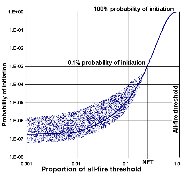
The shape of the distribution is not generally known, and use of a variety of statistical distributions including normal, log-normal and logistic distributions have been proposed. However, without an excessive sample size, the exact distribution cannot be determined and the tail is not well defined. Safety considerations generally demand a probability of initiation as low as 1×10⁻⁶—well down the tail of the distribution. As this cannot be determined from characterisation data, an appropriate safety margin is applied to the known data—the NFT stimulus.
Figure 6 shows the relationship between the stimulus pulse width and the energy needed to cause initiation. For firing current durations significantly less than Tc, there is no time for heat to flow into the bulk of the explosive and the EED will be sensitive to the energy dumped into it. For durations longer than Tc, there is time for heat flow to occur. Cooling will occur as energy disperses through the explosive and the EED will be sensitive to the applied power.
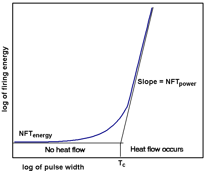
Radar transmissions are generally short widely spaced pulses with microsecond durations, so the average power is much less than the peak power. CC EEDs having values of Tc of a few microseconds can respond to individual radar pulses, and peak power needs to be considered. As the Tc for BW EEDs is generally several milliseconds, they do not respond to individual radar pulses, but rather to the average power.
Dudding
Dudding refers to the permanent degradation of the firing characteristics of an EED following application of stimulus insufficient to cause initiation. This can result from local heating modifying the characteristics of the explosive close to the bridgewire, from damage or burn-out the bridgewire, or, in the case of a CC device, from burning out of the shorter conductive paths. As EBW EEDs respond to the explosion of the bridgewire rather than its temperature rise, if insufficient energy is applied to cause initiation, it is possible to burn out the bridgewire, rendering the EED inoperable. For this reason, EBW EEDs sometimes have a spark gap included in their firing leads to isolate the bridgewire from any low-energy stimulus that may otherwise lead to dudding.
The possibility of dudding also has an impact on the firing strategies used to characterise EEDs. Because of the firing characteristics of an EED may be changed by testing it, during characterisation each EED can only be assessed once, regardless of whether it initiates or not. This significantly increases the sample size over that would be otherwise needed for characterisation. In general, no information exists on dudding thresholds, making the effects of dudding hard to include in assessments.
EED characteristics and applications
The principal electrical characteristics representative of different EED types are summarised in Table 1.
Because of their characteristics, the different EED types find different applications.
- BW EEDs are low-cost devices, and generally well characterised. Most have a low output, and are used to initiate explosive trains in general-purpose applications where initiation speed and precision are not critical. They only require a simple, low-voltage firing circuit.
- CC EEDs are more expensive, and have a wider spread of characteristics. They have moderate output and are generally only used where high-speed operation is essential. The firing voltage required is generally higher than for BW EEDs, but because of their higher resistance, firing circuits are not complex. Because of their low firing energy, high resistance and rapid response, they are more susceptible to electrostatic discharge and need to be handled with care.
- The EBW EED is a more expensive device, and only used in critical applications needing reliability, fast response and higher immunity to EEH. They require a high-energy firing pulse, usually generated by a capacitor discharge system and its associated circuitry, and this complexity increases the cost of the EO. They were originally developed for the precision initiation of multiple charges associated with nuclear devices. Spark gaps are sometimes included in series with the wiring within the EED to prevent low voltages reaching the bridgewire, thus providing enhanced immunity to EEH and dudding.
The electromagnetic environment
The EME to which EO can be subjected during its life can be very complex. P101 lists the following phenomena:
- Electromagnetic radiation (EMR)—the fields generated intentionally or unintentionally by radio, radar, and other equipment. EMR, or more particularly speaking, electromagnetic fields will induce currents on all conductive structures on which they are incident. Without proper management currents so induced in firing or control circuitry can lead to uncommanded initiation or disruption of EO.
- Electrostatic discharge (ESD)—generation or induction of electrostatic energy on, or inadvertent connection of charged objects to firing circuitry. ESD generally arises from friction, which causes a charge separation, leading to high electric potentials being induced on objects. Poor choice of materials, particularly plastics, can exacerbate the problem. Unless an appropriate discharge path is provided, electrostatic charge can find its way into firing circuits with damaging or disastrous results.
- Electromagnetic pulse (EMP)—the electromagnetic energy from a nuclear event, or from some directed energy weapons. EMP consists of a very short, extremely high pulse of electromagnetic energy. Because of the pulse shortness, its wide spectrum together with the high field strengths allow it to couple significant energy into structures that would otherwise be immune to EMR.
- Initial nuclear radiation (INR)—effects of short-time nuclear radiation (gamma rays) on electronics. Such radiation can temporarily or permanently modify the characteristics of semiconductor devices associated with firing circuits, and if such devices provide critical functions in the control of EO or weapon systems, hazardous situations may result. INR is also known as TREE (transient radiation electromagnetic effects).
- Lightning—coupling of energy into firing circuitry arising from a lightning strike on or nearby the EO. Energy may enter systems either as part of the lightning discharge current flowing through the EO system and its wiring, or as a result of the electromagnetic fields generated by the discharge current which can induce currents in the wiring.
- Electrical transients—energy coupling into firing circuits from switching transients in nearby cables. High switching currents in cables adjacent to firing leads can induce significant currents in the firing and other control leads and may lead to hazardous situations.
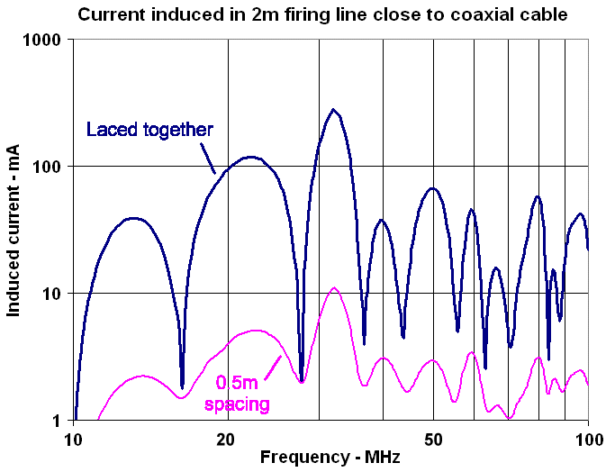
- Low-frequency magnetic fields—energy coupling into firing circuits from magnetic fields around nearby cables. Alternating currents can couple significant energy into adjacent firing and control leads leading to hazardous situations. This phenomenon is not limited to power frequencies, but can also occur at radio frequencies when antenna cables are run close to firing leads.
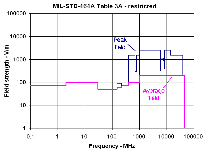
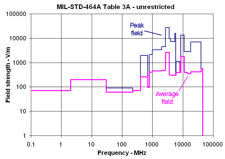
To provide a basis for the assessment in electromagnetic fields, EO is generally assessed against a particular radio-frequency environment. These environments are generally presented as tables of field strength versus frequency and are intended to represent the highest electromagnetic fields to which EO could reasonably be expected to be exposed during its life. They are the levels in which EO and its systems should be designed to remain safe, and are referred to as Minimum Service Radio Frequency Environments (MSRFE). The actual electromagnetic environment will evolve as new transmitting equipments and systems are introduced, and over the years a number of MSRFEs have been proposed. Probably the most recent is that published as Table 3A of MIL-STD-464A [4] which lists average and peak field strengths for restricted and unrestricted electromagnetic environments for EO. These environments are shown graphically in Figures 7 and 8 respectively. The lower restricted environment applies to assembly and loading of EO, while the unrestricted environment applies to all other phases.
The above environments purport to be representative of the field-strengths at some (unspecified) distance from radiating antennas. While assessment against such environments provides a starting point, it does not guarantee that the EO will remain safe in all situations. While EO may be assessed as ‘safe’, ‘susceptible’, or ‘unsafe’ in a particular environment, most assessments are only based on the EO in isolation. Susceptibility, however, is not only a function of the electromagnetic environment, but also the configuration of the EO and what may be attached to it. Different EO configurations from those for which an assessment has been made may have very different susceptibilities. The following are some possible examples:
- Removal of a missile from its transit case. The case may be designed to provide electromagnetic screening necessary to ensure that the EO is safe in transit.
- Handling of EO. Some EO has exposed firing contacts. An errant finger can significantly enhance pickup from the electromagnetic environment, leading to a hazardous situation.
- Loading of EO into its weapon system. It may be possible for the firing contact to touch part of the weapon system during loading. This, together with the ‘antenna’ effect of the handler could cause a hazardous situation.
- Connection of test equipment to EO. Unless properly designed, connection of test equipment to EO can provide a path for electromagnetic energy to couple into critical circuitry.
Field strengths higher than the MSRFE are often found close to antennas. Knowledge of the transmitter power and the antenna gain (that is, the proportion of transmitted power that is radiated in any direction) is not sufficient to estimate the fields close to the antenna as it does not include energy in non-radiating fields. Re-radiation from nearby structures, which will include the structure’s non-radiating fields, can also produce high field strengths in unexpected places.
It can be difficult to design EO systems that remain safe in such high field strengths. Because of this there is some pressure to assess land-based EO against a less severe environment such as are given in MIL-STD-464A for non-EO systems. However, in a world where land systems often find themselves shipboard, it is prudent not to do so. Different types of transmitting equipment and frequency usage can lead to unexpectedly high fields during coalition operations in the land environment. In addition, recent measurements have shown that MSRFE levels can be exceeded on the top of some military vehicles, particularly when more than one transmitter is operating.
Assessment against different environments would require that each susceptibility classification carry with it information on the assessment environment against which it was made. This has great potential for confusion, and could inadvertently lead to hazardous situations.
Electromagnetic fields
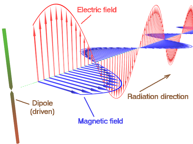
The electromagnetic fields associated with transmitting equipment consist of both electric and magnetic fields that vary in time and space. Some distance away from the radiating antenna and other objects, the radiating fields will consist of an electric and magnetic field at right angles to each other and to the direction of propagation. This is known as the far field region.
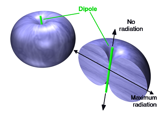
Figure 9 shows a single line of radiating electric (vertical) and magnetic (horizontal) fields at a distance from a tuned dipole antenna. A dipole antenna consists of a single wire driven at its centre. It is tuned when it is approximately 0.5 wavelengths long at the frequency of interest. As time proceeds the fields will travel towards the right. Figure 10 shows the distribution of radiating energy—the radiation pattern—at a significant distance from a dipole. The radiation pattern is three-dimensional and has the shape of a doughnut, with maximum gain radiated at right angles to the antenna axis—the direction of current flow, and no radiation along the axis of the dipole. Other antennas can have quite different radiation patterns.
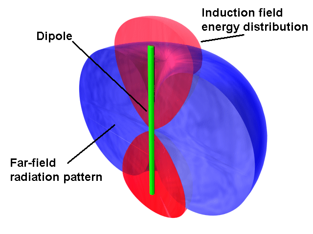
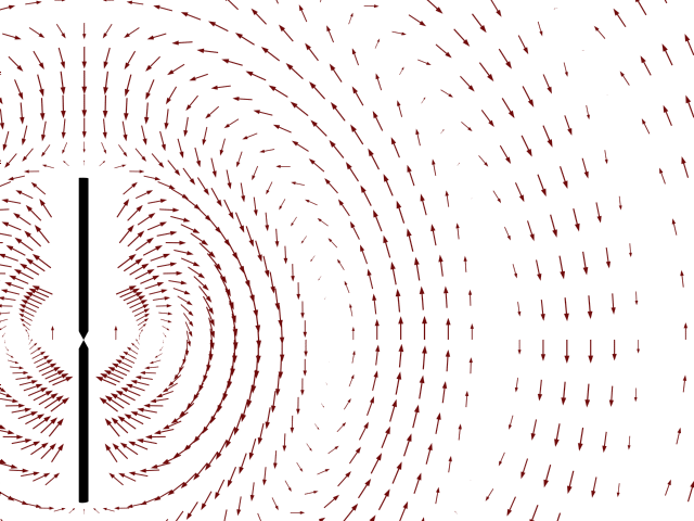
Figures 11 and 12 show the situation close to the antenna, in what is called the near-field region. This region contains both radiating and non-radiating, or induction, fields. While energy in the radiating field travels away from the antenna, energy in the induction field flows back and forward from the antenna to the surrounding region. Both types of field are capable of inducing currents in structures within their region of influence. For small antennas the notional boundary of the near field region is λ/2×pi, where λ is the wavelength of the radiation. This boundary represents the distance at which the energies in the radiating and non-radiating fields are approximately equal. While the strength of the induction field decreases at a greater rate than the radiation field, it is not zero outside the near field boundary. In addition, the spatial distribution of the induction field is quite different from that of the radiating field, being a maximum at the ends of the dipole. Because of this, the use of antenna gain data to predict field strength distributions is only valid providing that the induction field is negligible—and that means at many times the near-field boundary distance. This can be hundreds of metres for low-frequency or high-gain systems—generally well outside the area for EEH problems.
Nearby conducting structures will also have a significant effect on the field distribution, often producing high field strengths at unexpected locations. Figure 13 shows an FFG with a high-frequency (HF) transmitting antenna at the rear port location.
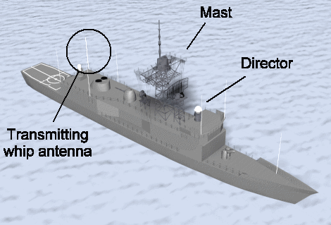
Figure 14 shows a cross-section of the electric field strength distribution from that antenna at 30 MHz. Note the regions of enhanced field strengths some distance from the transmitting antenna. These result from re-radiation from the mast and director structures, which happen to be resonant at that frequency.
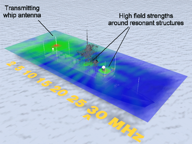
Another issue, particularly in the HF band (2–30 MHz) is that the radiated power can vary considerably from the published data. Because of such effects, it is prudent to conduct a survey of field strengths for the particular configuration, and indeed P101 requires that an assessment be undertaken to determine hazards in the actual platform environment.
Coupling and susceptibility reduction
An electromagnetic field can couple energy into any conducting objects on which it is incident. The shape, size and orientation of a wire and the wavelength determine how much energy is coupled. Figure 15 shows energy coupled into a passive dipole—an actual antenna, or just a piece of wire. Coupling will be maximum with the wire parallel to the electric field and less if the wire is at other angles. Figure 16 shows the orientation of a loop of wire for maximum coupling, with the plane of the loop at right angles to the magnetic field. Other angles will produce lesser coupling. Coupling is also greatly affected by the dimensions of the object relative to a wavelength (λ). For the dipole, maximum coupling will occur if its length is just under ½ λ; for the loop when the circumference is equal to λ. Figure 17 shows how untwisted leads on a blasting cap can form a dipole antenna. The most hazardous situation will arise if the dimensions are close to ½ λ.
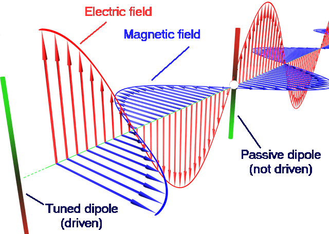
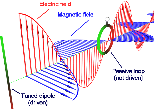
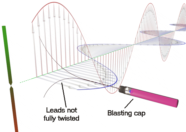
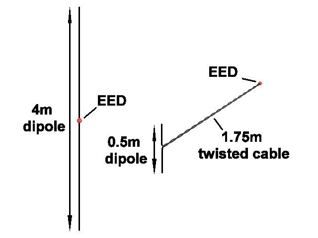
Figure 18 shows a 4m length of wire with an EED at its centre—as a 4-m dipole and a ½-m dipole with the remainder of the wire as a twisted cable. Figures 19 and 20 show the induced currents for these two configurations in a 100 V/m field, for the dipole parallel to the electric field (maximum coupling), and at an angle of 70° to it.
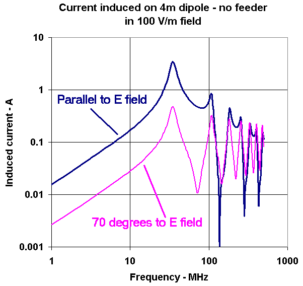
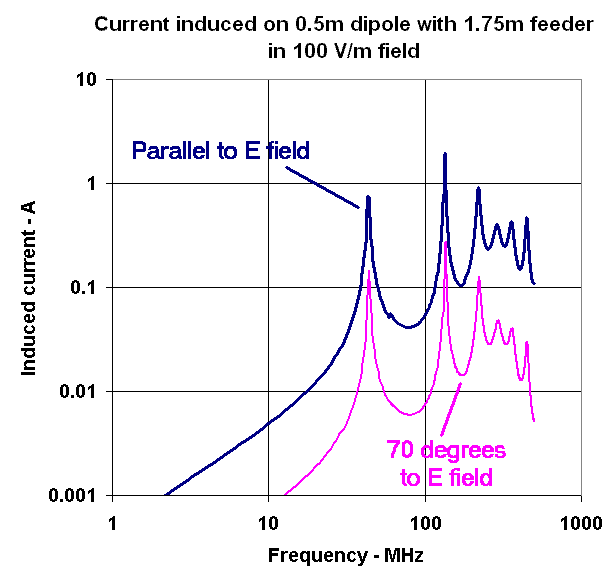
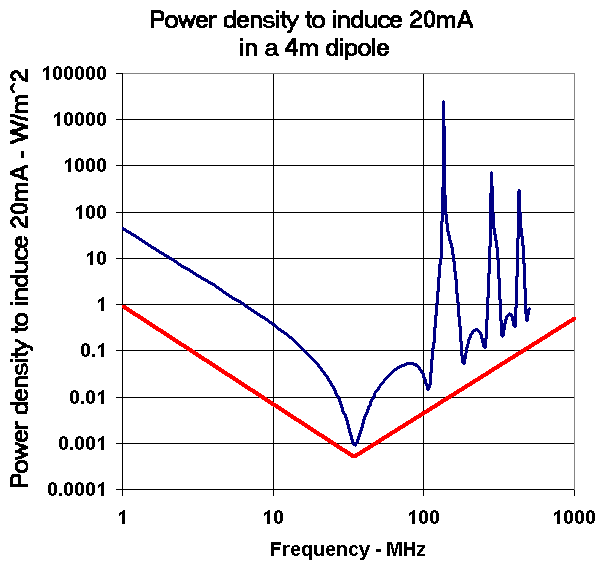
For the 4-m dipole, the first resonance occurs at 34.5 MHz, when the dipole length corresponds to just under ½ λ. The current induced in the dipole is greatest at this frequency, and if the dipole forms part of an EO firing circuit, the susceptibility will be the greatest. Rotating the dipole to 70° to the electric field significantly reduces the induced current at this frequency. Other resonances will occur when the dipole length is an odd multiple of ½ λ—that is, 3/2 λ, 5/2 λ, 7/2 λ and so on, the induced current being less for the higher order resonances. For the 0.5-m dipole and 1.75-m feeder, pickup at the first resonance is significantly reduced, although the second at 120 MHz is increased, probably as a resulting of the matching provided by the feeder.
| Range (dB) | Power ratio | Current/voltage ratio | |
|---|---|---|---|
| Trials factor Component variability System configuration Measurement/orientation Total (root sum of squares) | 2–10 3–10 3–10 4.6–17.3 | 1.5:1 to10:1 2.0:1 to 10:1 2.0:1 to 10:1 2.9:1 to 54:1 | 1.25:1 to 3.1:1 1.4:1 to 3.1:1 1.4:1 to 3.1:1 1.7:1 to 7.3:1 |
| Safety margin (reliability/safety) | 3–10 | 2.0:1 to 10:1 | 1.4:1 to 3.1:1 |
| Total (best case—well characterised and documented) | 7.6 | 5.8:1 | 2.4:1 |
| Total (worst case—very little information) | 28 | 630:1 | 25.1:1 |
Safety factors and trials margins
P101 gives a flexible approach for the derivation of a safety factor based on the variability of a number of parameters of the EO. This not only looks at the rigour of EED assessment, but the variability of wiring, system orientation, and measurement uncertainty.
EEH assessments fall into two categories—reliability assessments and safety assessments:
- Reliability assessments apply to those situations where the consequences of inadvertent initiation or firing circuit malfunction are non-hazardous. The threat level at which there is an acceptably low probability of malfunction is determined, often by theoretical methods. To this level is added a margin to account for uncertainties such as component variability (NFT, for instance). This is called the variability margin. Where the level is determined by other means, including physical trials, a further margin is added to allow for measurement uncertainties, including the effects of orientation, test frequency, and spacing. This, combined with the variability margin is called the trials factor.
- Safety assessments apply to those situations where the consequences of an incident are hazardous. In addition to the variability margin or trials factor, a safety margin is added to reduce the probability of a malfunction to a level appropriate for safety considerations.
Margins are based on the information available, the test facility, and the nature of the hazard. Table 2 is derived from the recommendations of P101.
The US Navy’s HERO methodology applies a fixed safety factor of 16.5 dB (45:1 power ratio or 6.7:1 current/voltage ratio). While this lies within the range of the P101 limits, without prejudicing safety, the flexibility of P101 can result in less draconian restrictions in deployment of EO.
Assessment methodologies
There are a number of methodologies that are used to perform EEH assessments. Confidence in the results is generally proportional to the effort needed in performing the assessment.
- Estimation by inference. This method compares two items of EO of similar design, one already having been assessed. The usefulness of this method depends on the significance of the differences between the two items of EO (or EO systems), and the rigour of the initial assessment.
- Go-NoGo testing. This method uses an item of EO with the explosive removed, but EEDs and their circuitry intact. This EO is then tested by exposing it to the environment for which the assessment is being made. The rationale is that if an EED is initiated then there is a susceptibility problem. What cannot be said is that if an EED does not initiate, there is no susceptibility problem. There is no way of knowing how close the EED came to initiation or indeed, where the EED sensitivity fell in the firing distribution. Fitting of a more sensitive EED can improve the situation, but that may not be possible if the initial EED is already a sensitive type. Exposure to a higher field than the MSRFE will also assist, but it is unlikely that such a high environment would be available. It may also introduce non-linear effects such as filter saturation and arc-over, invalidating results. A further uncertainty is introduced by the possibility that dudding will have modified the EED characteristics during previous testing. This method cannot demonstrate that the EO is safe, and produces little more than a comfortable feeling that something has been assessed so that a tick can be placed in the box.
- Theoretical methods. P101 includes a theoretical method which is of considerable use in performing a ‘first-pass’ EEH assessment of bare EO in an RF environment, in particular the MSRFE. It involves reduction of the wiring associated with the EED, including generic wire layout and dimensions, screening, and shielding, to its bare essentials, to generate a plot of the maximum safe field against frequency. The graphs of Figures 19 and 20 showed the current induced in dipoles of different configurations in a known electromagnetic field. The same data can be plotted as the power density that will induce a specified current in an EED connected at the centre of the dipole. While this is possibly the most susceptible configuration for an EED, it does serve to illustrate the theoretical method of P101.
Figures 24 and 25 show the power density (assuming far field conditions) that will induce 20 mA in an EED connected to the centre of a wire. The examples are for the same configuration shown in Figure 18, namely a 4-m dipole, and a 0.5-m dipole plus 1.75-m feeder. For each configuration, a worst case envelope has been plotted as a minimal series of straight lines. The sloping lines have a slope of 20 dB per decade—that is, a 100:1 change in power density for a 10:1 change in frequency. Without going into the mathematics involved, this slope is a consequence of the physics of electromagnetic coupling. The theoretical method embodied in P101 is based on this and related strategies, and from a specified wiring geometry, calculates the shape of the worst-case envelope. The algorithms necessary to calculate this envelope have evolved from data on a large number of physical measurements on a variety of different wiring configurations. A computer program “Electromagnetic Analysis Software” (EAS) embodying these techniques has been developed in UK.
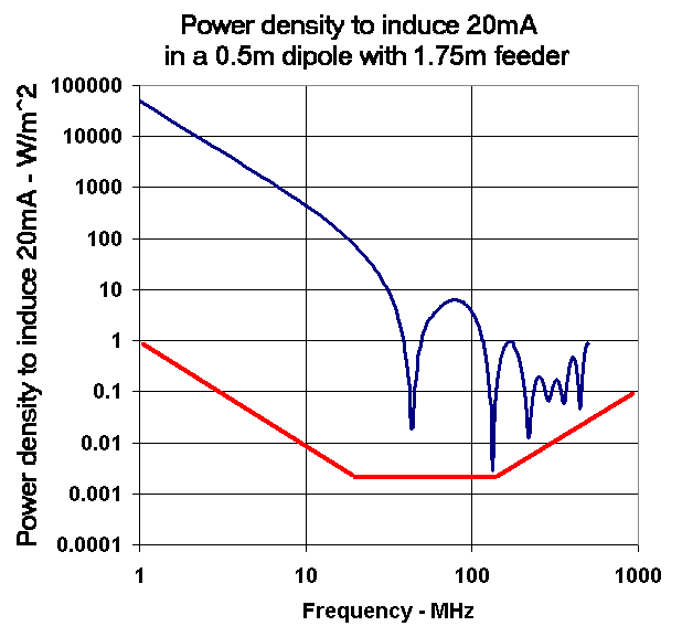
Because EAS works from a grossly simplified representation of the wiring and represent the worst case, the results are necessarily conservative. However, EAS does provide a fast indication as to whether the EO can be considered ‘safe’, or whether further assessment needs to be made. Because of the minimal wiring configurations that can be accommodated, in general this method will not address the additional effects that result from a weapon system when the EO is loaded. Nor will it address effects of handling or cable-to-cable coupling on firing systems and to address these aspects instrumented trials are generally required.
Figure 26 shows the windows provided by EAS. General assessment parameters and the MSRFE are entered or selected in the Environment window. Wiring geometry and other configuration data are entered in the Circuit window. The susceptibility envelope and the selected MSRFE are shown in the Results window. This particular example is for a 3-m single wire and includes some cable screening and a shield containing a gap. This results in the quite complex shape of the susceptibility envelope. Hazards are indicated where the susceptibility envelope falls below the MSRFE—in this case, frequencies from about 30–700 MHz and 1,200–12,000 MHz—not a good electromagnetic design!
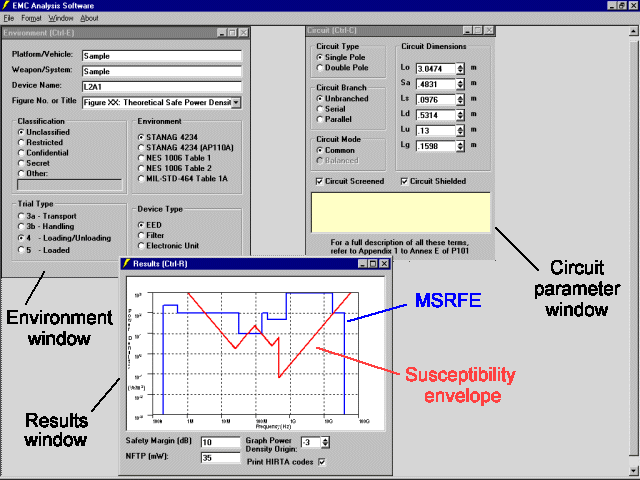
Figure 27 shows one of many screens from AussieEAS, Land Engineering Agency’s enhancement of EAS. Apart from a greater range of screen options, this tool includes the following enhancements and extensions:
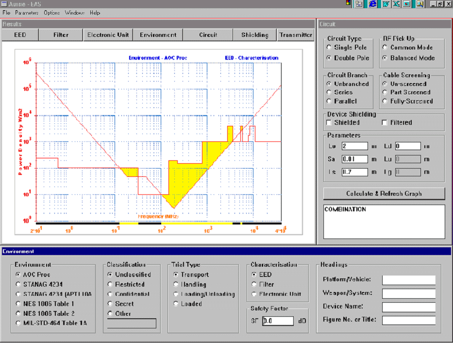
- a database of EED characteristics, including user-defined EEDs;
- a more extensive range of MSRFEs, including a user-defined environments,
- extensive help in the form of wiring topology drawings based on illustrations contained in P101;
- a database of transmitter data;
- a safe-distance calculation; and
- import/export of susceptibility data and configuration description for use in other applications.
Detailed electromagnetic modelling. There are a growing number electromagnetic modelling strategies and software tools that address a wide range of electromagnetic problems. These can be used to gain valuable insight into the behaviour of EO and associated systems, however, the limitations and range of applications of the various tools need to be thoroughly understood. With properly validated models, they can be used directly to investigate EO susceptibility. Modelling is also of great benefit in support of other assessment techniques, particularly in the reduction of the number of measurements needed for instrumented trials. Prior determination of resonant frequencies and orientations for worst coupling can guide trial strategies to focus time, effort and spectrum in those measurements that will yield the most valuable information. In some circumstances up to a 90% reduction in effort can be obtained.
Instrumented trials. Instrumented trials involve the exposure of EO and systems, free from all explosive content and containing only the EED electrical components and their associated circuitry. Specialised instrumentation is built into the EO to measure pickup during exposure. Not only does the instrumentation require extreme sensitivity, resolving fractions of a °C change, but also it must not modify the pickup by its presence. For BW EEDs, the parameter measured is the bridgewire temperature rise, and this needs to be done without any electrical contact with the bridgewire.
Over the years a number of different temperature sensors have been used, ranging from paints that change colour with temperature, to electrical sensors. These include:
- microscopic thermistors (temperature sensitive resistors);
- thermocouples (junctions of dissimilar metals that produce a voltage in response to temperature change); and
- thermopiles (arrays of thermocouples).
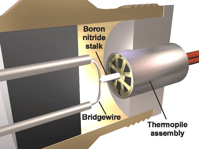
Such devices are thermally bonded to the bridgewire with an electrically insulating material such as beryllium-oxide paste or a boron-nitride rod. A suitable electronics package fitted within the EO translates the temperature information into a form that can be transmitted by non-electrical means such as a fibre-optic cable. This isolation is necessary to avoid any external electrical connection to the instrumentation package, which could modify the electrical pickup system, invalidating results. Figure 28 shows a thermopile fitted to a BW EED.
Electrical temperature sensing can have problems at microwave frequencies when the proximity of common-mode voltages on the EED can induce currents in the sensor, which it erroneously interprets as a temperature rise. Great care needs to be taken to strike a balance between sensitivity and common mode immunity.
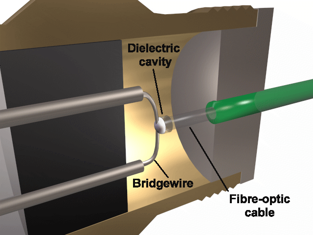
A comparatively recent innovation in non-electrical temperature sensing with sufficient sensitive for EEH work involves the use of a dielectric material with a refractive index that changes with temperature. A small cylinder of this material is sandwiched between two mirrors, and is called a cavity. The cavity is bonded to the end of a fibre-optic link and thermally connected to the bridgewire. Optical interferometry is used to measure the time taken for light to pass through the dielectric cavity, which is related to the temperature of the dielectric material. Figure 29 shows this instrumentation fitted to a BW EED. This system offers much simplicity over conventional instrumentation methods as it does not require the development of an electronics package within the EO. It should also provide immunity against electromagnetic effects such as common-mode response.
Instrumentation of CC EEDs presents some special challenges. Although initiation is a thermal effect, it is on a microscopic scale, and can occur anywhere within the bulk of the explosive. Consequently, it is not possible to use thermal sensors such as are used with BW EEDs, and the voltage is the only parameter that can be measured. Special high-impedance voltage measurement instrumentation is required to measure the voltage with minimal loading on the firing circuit. The frequency response of the instrumentation also needs to be sufficiently high that it will accurately read voltages up to the frequency of interest—generally well into the GHz range. These two requirements conflict, and compromises need to be made in one or both of them. Further discussion is outside the scope of this paper.
P101 requires EEH assessment in the electromagnetic environment of the platform. In many instances, this can exceed the MSRFE against which an item of EO has been cleared. If the EO is to be used with a platform-mounted weapon system there could be additional wiring introduced that is not part of the original EO system as assessed. As noted previously, wiring other than that associated with the EO can impact on the susceptibility performance. Theoretical methods are of little use and an instrumented trial using the platform’s emitters is needed. The effect of apparently innocuous wiring changes on EO susceptibility implies that careful configuration control of the whole platform is required to maintain safety.
Frequency and orientation steps
The current induced in a given EO or EO system will be a function of the frequency of the radiation and the orientation of the EO relative to its polarisation. For all detailed assessments, whether they involve electromagnetic modelling or physical measurement using instrumentation, it is essential to see that either:
- enough allowance is made in the measurement/orientation component of the trials factor, or
- that enough frequencies/orientations are evaluated so that the worst case is found.
Figure 30 shows the susceptibility curves for the 4-m dipole, using three different frequency-step strategies, each covering 1–500 MHz.
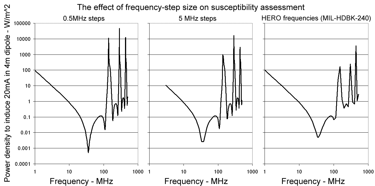
The spread of the above predicted “safe” power densities illustrates the importance of frequency resolution and its effect on susceptibility assessment, particularly at around resonances. However, measurements are costly and it is clearly desirable to minimise the number without compromising data integrity. If the approximate shape of the susceptibility curve were known prior to the test run, for instance, from detailed electromagnetic modelling, a minimum frequency set could be developed so that measurements would yield the most useful information. Alternatively, a manual real-time adaptive frequency selection strategy could be implemented by plotting susceptibility measurements as the assessment proceeds, and observing the critical frequencies as they become evident. Observing measurement trends, initially at widely spaced frequencies, would allow progressive homing in on the critical regions. Test effort can also be significantly reduced by computer-based control and data logging, particularly if implemented together with an intelligent test frequency selection process such as that offered by Model-Based Parameter Estimation [5]. Because test frequencies are only determined as the testing proceeds, such adaptive frequency strategies would require significant co-operation between the testing and spectrum management agencies.
EEH test facilities and instrumentation sensitivity
Production of electromagnetic fields approaching the MSRFE, particularly over larger volumes such as that of military vehicles, requires a very significant investment in test facilities. The HF and low VHF bands (2–80 MHz), generally require an open-air site, but there is considerable resistance to the large expenditure involved. It should be noted, however, that in addition to EEH, such a facility would also address the electromagnetic vulnerability of vehicles and other systems in a full threat environment, the hazards of which are currently ignored—with some interesting consequences.
| Strategy | Data points | Worst frequency | “Safe” power density |
|---|---|---|---|
| Linear steps of 0.5MHz, starting at 1 MHz | 1,000 | 34.5 MHz | 0.0005 W/M2 |
| Linear steps of 5 MHz, starting at 3 MHz | 100 | 38 MHz | 0.0026 W/m2 |
| “HERO” frequencies from MIL-HDBK-240 | 57 | 36 MHz | 0.005 W/m2 |
Exposure to a lesser environment and extrapolation of the results might seem an attractive proposition, as it would require significantly less investment in facilities, as well as being less electromagnetically anti-social. However, there is a limit to the amount of extrapolation that can be applied and still obtain meaningful results.
Figure 31 shows a typical situation with a BW-based EO system. The graph shows the probability of initiation versus current induced in the firing circuit. The all-fire threshold is around 500 mA, and the no-fire threshold is 200 mA. A safety margin and trials factor is then applied. Depending on how well the EO system is defined, this could be between 7.6 dB and 28 dB. For 28 dB, this gives a maximum safe current of 20 mA.
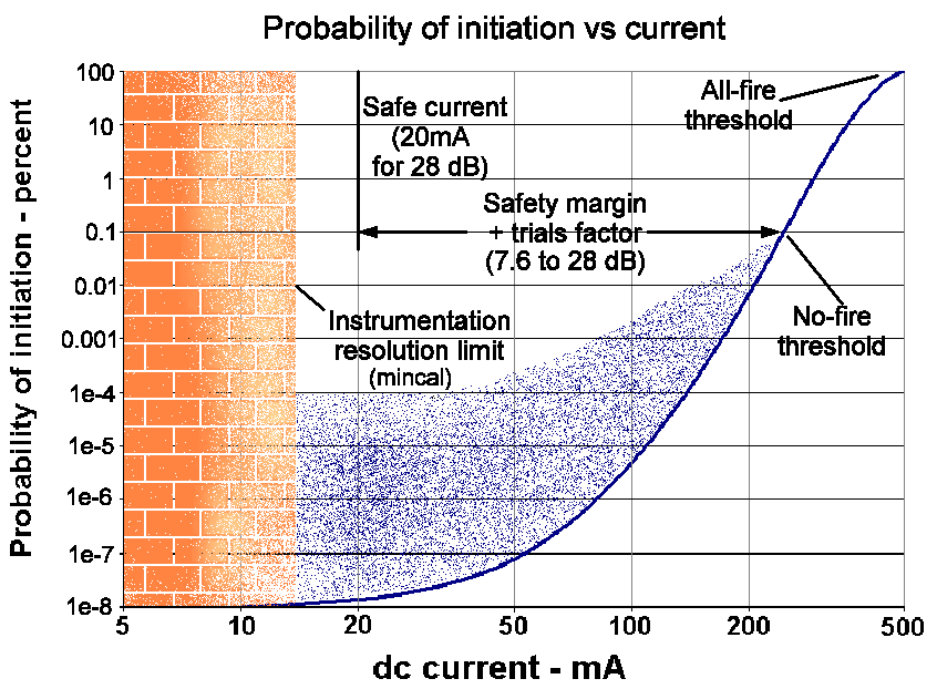
The resolution limit of the instrumentation is called the mincal. This limit is imposed by the noise floor of the instrumentation, and readings at or below this level can only be assumed to be at the mincal. The best instrumentation currently available has difficulty resolving currents much below about 10 mA.
The degree of extrapolation that can be applied depends on the difference between the safe current and the mincal. If EO without any pickup were exposed to (say) 55 V/m, a reading equal to the mincal would be obtained, pickup equal to the mincal would be assumed. If the mincal were 10 mA, extrapolating from 55–100 V/m would give 18 mA, just under the safe limit of 20mA, and the EO would be assessed as safe. However extrapolation from 55–200 V/m, would give 36 mA, and the EO would be assessed as unsafe. This may lead to unnecessary operational restrictions being imposed on the use of the EO. Extrapolation of instrumentation noise just yields more instrumentation noise. A greater degree of extrapolation would be allowable if the EO were better defined, allowing a lesser safety margin+trials factor, or more sensitive instrumentation with a lower mincal were available. Exposure to the full threat environments will also ensure that non-linear effects such as arc-over and saturation of filters are evaluated. Clearly, exposure to the full threat environment is the ideal.
Assessments of fire-control units. Fire-control units (FCUs) are elements of an EO system that issue firing commands to the EO. They range from simple switch and relay circuits to complex electronics and microprocessors. While there is little likelihood that switch and relay systems will be susceptible to electromagnetic threats, those with electronic components can be very susceptible. Without careful design, the electromagnetic environment can cause electronic systems to malfunction, leading to significant hazards. There is little point in ensuring that pickup on firing leads is acceptably low when the same environment confuses the FCU electronics so that it issues a firing command. Like Go-NoGo testing of EO, seeing if the FCU malfunctions when exposed to the EMR is of limited value. Evaluations require instrumentation embedded in the FCU itself that is capable of detecting levels well below the switching thresholds of the electronic devices. Without this there is no knowledge of how close the FCU was to malfunction.
Conclusions
This paper has provided some background on EEDs and their characteristics, on the electromagnetic environment, particularly electromagnetic fields, and the coupling mechanisms between the two. Both theoretical and practical assessment techniques and strategies including the associated trials margins and safety factors have been discussed. The importance of obtaining sufficient data to resolve worst case scenarios has been stressed. While there are many other aspects of EEH that are not here addressed, it should provide the novice some insight into the mysteries of electro-explosive hazards, and useful background for the select few who may enter the field, or those who may be effected by their assessments.
References
[1] P236.94: Guidelines for the Preclusion of Electro-explosive Hazards in the Electromagnetic Environment, Australian Ordnance Council Pillar Proceeding, 27 October 1994.
[2] P101 (issue 2): Principles for the Design and Assessment of Circuits Incorporating Explosive Components, UK Ordnance Board Pillar Proceeding, 29 April 1997.
[3] MIL-HDBK-240: Hazards of Electromagnetic Radiation to Ordnance (HERO) Test Guide, US Department of Defense, 1 November 2002.
[4] MIL-STD-464A: Electromagnetic Environmental Effects Requirements for Systems, US Department of Defense, 19 December 2002.
[5] E.K. Miller and T.K. Sarkar, “An Introduction to the Use of Model-Based Parameter Estimation Electromagnetics”, Review of Radio Science, 196-199, R.Stone (ed), August 1999, pp. 139–174.