Volume 9, Number 3, November 2006

Optimal Path Trajectories In A Threat Environment

Harvinder S. Sidhu¹, Geoffry N. Mercer¹, Mary J. Sexton², and Nadeem A. Ansari¹

¹ School of Physical, Environmental and Mathematical Sciences, University of New South Wales at the Australian Defence Force Academy, Canberra, ACT 2600, Australia.
² Belconnen , Canberra, ACT, Australia.

Abstract

Minimizing the risk of detection in a hostile environment is a fundamental requirement of all military operations. Often the trajectory of a vehicle is dependent on other factors such as maximum travel time, fuel usage, and the like, which provide constraints on determining the optimal path of the vehicle. The risk to the vehicle is from detection and subsequent action by enemy forces. Often this detection is from radar. Here we investigate the single vehicle path planning problem to minimize radar exposure. We formulate the problem in a continuous way and present numerical results for a single threat radar. We also show how our approach can be extended to include a second threat radar. By extending our approach we believe that a feasible technique to determine the optimal path in a threat environment consisting of a network of multiple threat radars can be obtained, perhaps even undertaken by on-board systems.

Introduction

Background

Murphey et al [1] note that determining the optimal path trajectory is a fundamental requirement for land, naval, air, and space vehicles in both military and civilian applications. Very often these applications also include constraints on resources (such as fuel usage). A number of objectives and constraints on resources are given in [1,2] and these include: minimizing the risk of aircraft detection by enemy radars, sensors or surface-to-air missiles (SAMs); minimizing the risk of submarine detection by sensors; determining the optimal trajectories for multiple aircraft in an air-traffic-control environment; maximizing the probability of target detection in surveillance operations; minimizing the consumption of propellant by a spacecraft in interplanetary and orbit transfers; minimizing the fuel and time cost for commercial planes, and minimizing the energy requirement for a unmanned automated vehicle. Each application would seek a different balance and can afford different levels of risk. Researchers are continually investigating different methods to determine the “optimal” paths from start to finish while attempting to minimize each problem’s associated risks.

Motivation and scope

This paper investigates the determination of optimal path routes for a single air vehicle flying from its base (point A in Figure 1) to its mission objective (point B) when the flight path is through an area containing enemy radar installations. We study this problem in a continuous variable setting—in other words, we allow the course of the aircraft to be continuously changing in order to minimize the risk of detection. This is in contrast to previous work in this area such as [1], [3–5], who have all treated the aircraft trajectory as a series of discrete steps and used discrete optimization techniques on this approximate problem (see Figure 1). A serious drawback of such a discretization approach is the determination of suboptimal paths due to the gridding scheme incorporated in such methods [6]. One way to improve this is to increase the number of discretization points, but this is often not feasible (particularly for on-board systems) due to high computational costs.

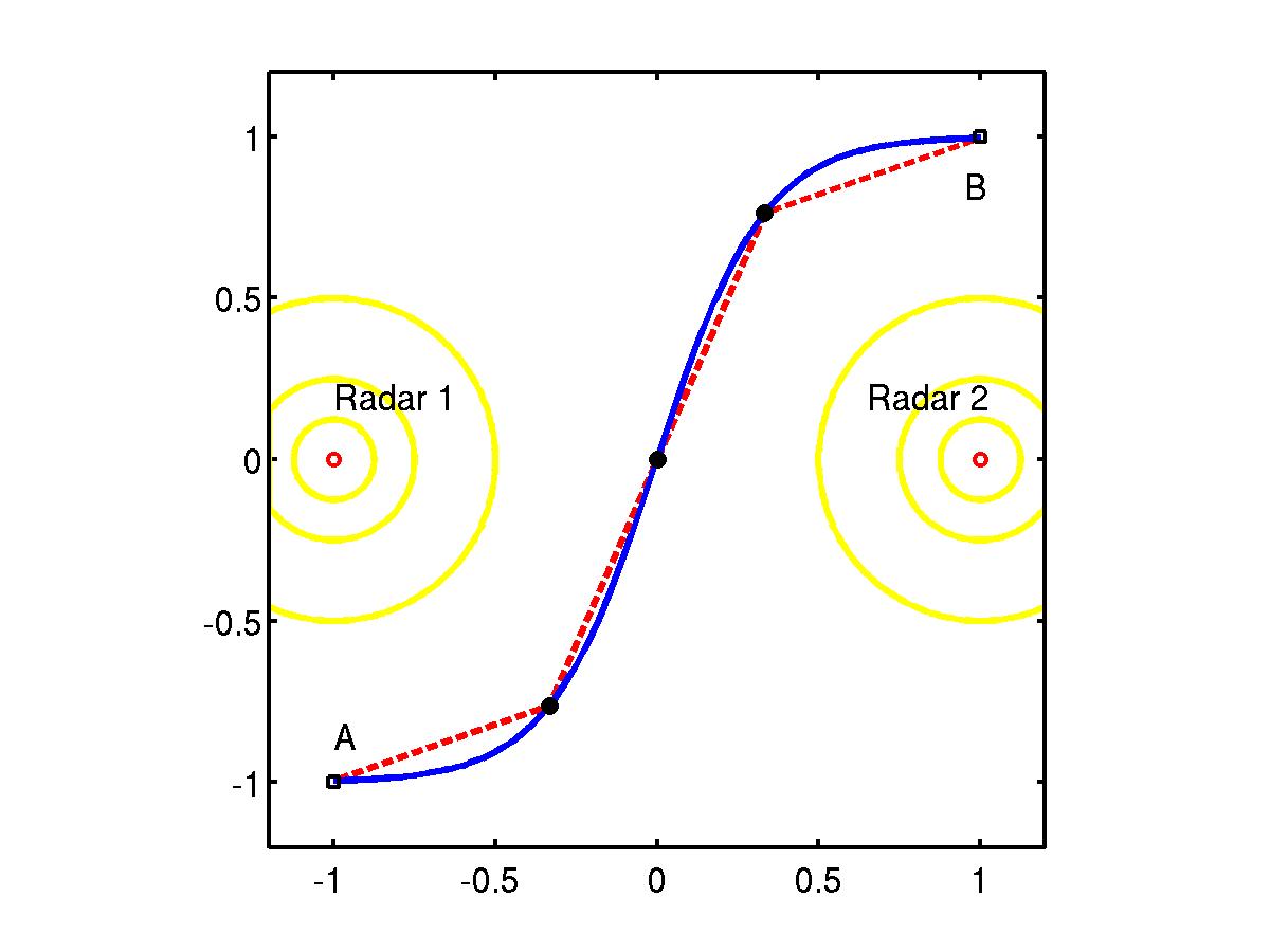
Figure 1. Schematic diagram showing an air vehicle flying in a hostile environment with two radars. Points A and B represent the location of the base and the mission objective respectively. The dashed line shows the discrete solution to the trajectory path whereas the bold curve joining points A and B shows the continuous solution.

Murphey et al [1] and Zabarankin et al [3] did consider the continuously varying formulation of the problem but only for the case of a single radar with very specific conditions that allow for analytic solutions and are not very practical. These were used to test their discrete optimization numerical schemes.

Some other methods that have been used to obtain optimal routes include: the Voronoi diagram search (see, for example, [7–10]); the modified A^* graph-searching technique [11]; the analogous problem formulation (for example, Bortoff [12] refines the initial polygonal path from the Voronoi approach by representing the path using the dynamics of virtual masses being acted on by both the spring restoring force and by the virtual forces pushing from each radar site); and the probability threat map [13].

Novy [6], on the other hand, employed several numerical schemes (both continuous and discrete) to investigate the single-radar problem. However this work was restricted only to the cases where analytical solutions of the problem were possible, namely the angle between the base, enemy radar and destination was between 0° and 60°. Novy’s two-radar trajectory optimization was also limited to exclude travel around radar locations. In this paper we investigate the problem numerically for the case of single radar without the previously used specific conditions that obviously limit the practical application of this study. We shall also discuss the case when our method is extended to the case of two radars and present some preliminary results for this scenario. The distinction in the approach described here is that previous techniques are heuristic based, that is an approximated algorithm (or colloquially, a ‘rule of thumb’) is used to determine, in general, sub-optimal solutions. Our approach depends on a numerical solution technique which itself is an approximation, particularly in discretization, however it is based on solving the equations exactly. Our aim is to show an approach which is amenable to standard differential equation solvers rather than a heuristic approach.

Problem formulation

Here we follow [3] and present the continuous formulation of the problem. As in most of the studies listed in the reference, we shall assume: (i) air vehicle travels with constant speed; (ii) position of air vehicle is considered only in the horizontal plane; and (iii) radar detection does not depend on the air vehicle’s heading and climb angles (in other words the radar cross-section (RCS) of the vehicle, which can vary as much as two orders of magnitude in flight, is assumed to be constant, see [14] and [15]). The main purpose here is to understand and gain important insights into the fundamental problem without these additional complications.

Consider the case of N radars at positions (x,y)=(a_i,b_i) for i=1…N. The vessel starts from its base, point A=(x₁,y₁), and moves to its destination, point B=(x₂,y₂) with constant speed. Let the trajectory of the aircraft be parameterized by the variable s (the arc length). The length of the trajectory l is therefore:

l = \int_{A}^{B} ds

(1)

The distance from any point (x,y) on the trajectory to the i^th radar is:

d_{i} = \sqrt{(x - a_{i})^{2} + (y - b_{i})^{2}}

(2)

According to Skolnik [16], the amount of power received by a radar can be expressed by the radar range equation:

P_{r} = \frac{P_{t} {GA}_{e} σ}{(4 π)^{2} d^{4}}

(3)

where P_t is the power of the radar transmitter, G is the transmitter gain, A_e is the effective area of the receiving antenna, σ is the radar cross section (RCS) of the target (here, the air vehicle), and d is the distance of the vehicle from the radar. Following [3] we shall assume that all the radar technical characteristics (such as the maximum detection range, the minimum detectable signal, the transmitting power of the antenna, the antenna gain, and the wavelength of the radar energy) remain constant. Hence the risk factor, w_i, for the i^th radar can be assumed to be a constant, and the risk index can be expressed as r_i=w_i/d_i⁴. This corresponds to Skolnik’s [16] radar detection model with a signal reflected from the aircraft. However in this paper we shall follow Zabarankin et al [3] and consider the risk as a reciprocal of the square of the distance. These authors have stated that “…such an assumption is not critical for the application of the developed methodology.” Furthermore since our objective of this paper is to highlight the usefulness of the continuous variable setting as opposed to discretizing the aircraft’s trajectory, and to compare our results with those reported in [3], we shall therefore follow [3] and assume that the risk index is r_i=w_i/d_i². It should be noted that under the numerical scheme presented here the case r_i=w_i/d_i⁴ can be easily accommodated by simply altering the relevant equation. The r_i=w_i/d_i² case is useful in that analytic solutions as those presented in [3] are possible under special conditions which provide a validation of the numerical scheme. The total risk R for the aircraft along the entire trajectory from the points A to B (from the base to the mission objective) can now be expressed as:

R = \int_{A}^{B} \sum_{i = 1}^{N} \frac{w_{i}}{d_{i}^{2}} ds

(4)

Following [3], using calculus of variation arguments, the equations that govern the risk associated with the radars can be expressed as a system of differential equations:

\frac{\partial L}{\partial x} - \frac{d}{ds} (\overset{}{\frac{dx}{ds}} L) = λ \frac{d^{2} x}{{ds}^{2}}

(5)

\frac{\partial L}{\partial y} - \frac{d}{ds} (\overset{}{\frac{dy}{ds}} L) = λ \frac{d^{2} y}{{ds}^{2}}

(6)

where λ is a constant of integration that needs to be found. By using Equation (2), the risk functional L appearing in the governing differential equations above can be expressed as:

L = \sum_{i = 1}^{N} \frac{w_{i}}{(x - a_{i})^{2} + (y - b_{i})^{2}}

(7)

Rearranging Equation (5) gives:

(λ + L) \frac{d^{2} x}{{ds}^{2}} = \frac{\partial L}{\partial x} - \frac{dx}{ds} \frac{dL}{ds}

(8)

A similar expression can be written for Equation (6). By letting z₁=x, z₂=dx/ds, z₃=y and z₄=dy/ds, it is now possible to express the governing Equations (5) and (6) as a system of four first-order differential equations, namely:

\frac{{dz}_{1}}{ds} = z_{2}

(9)

\frac{{dz}_{2}}{ds} = \frac{1}{λ + L} (\frac{\partial L}{\partial z_{1}} - z_{2} \frac{dL}{ds})

(10)

\frac{{dz}_{3}}{ds} = z_{4}

(11)

\frac{{dz}_{4}}{ds} = \frac{1}{λ + L} (\frac{\partial L}{\partial z_{3}} - z_{4} \frac{dL}{ds})

(12)

with

\frac{\partial L}{\partial z_{1}} = \sum_{i = 1}^{N} \frac{- 2 w_{i} (z_{1} - a_{i})}{[(z_{1} - a_{i})^{2} + (z_{3} - b_{i})^{2}]^{2}}

(13)

\frac{\partial L}{\partial z_{3}} = \sum_{i = 1}^{N} \frac{- 2 w_{i} (z_{3} - b_{i})}{[(z_{1} - a_{i})^{2} + (z_{3} - b_{i})^{2}]^{2}}

(14)

and

\frac{dL}{ds} = z_{2} \frac{\partial L}{\partial z_{1}} + z_{4} \frac{\partial L}{\partial z_{3}}

(15)

Since s is an arc length and the vehicle is assumed to be travelling at constant speed, there is also the additional constraint:

(\frac{{dz}_{1}}{ds})^{2} + (\frac{{dz}_{3}}{ds})^{2} = 1

(16)

Numerical method

Solving the governing Equations (9) to (12) numerically is a routine procedure for several types of boundary-value problems. The known and unknown quantities must first be identified, with the initial point (base) A=(x₁,y₁) and the final point (mission objective) B=(x₂,y₂) known. The slopes (dx₁/ds,dy₁/ds) and (dx₂/ds,dy₂/ds) at the points A and B are unknown, however Equation (16) describes the relationship between these slopes. Either one of the parameters λ or l is also an unknown (that is, choosing a value for one means the other is an unknown). There are essentially two approaches for solving this type of system of equations:

fix the length of the trajectory l and solve the governing equations to find the path of the trajectory and the corresponding λ that satisfies the equations; and
fix z₂(0) and solve the governing equations to find the trajectory including its length l that satisfies the equations.

During our implementation of the numerical method, we found that method (i) works better for trajectories close to a straight line, whereas method (ii) is more appropriate for large (wide) trajectories due to the sensitivity of the solutions to the parameters l and λ at these extremes. We use the Numerical Algorithms Group (NAG) [17] routine DO2HBF which is ideally suited to these types of two-point boundary-value problems with unknown parameters. The main requirement for this routine is that the number of unknown parameters must equal the number of equations. We have four differential equations (Equations (9) to (12)) therefore for a given trajectory length l, we can treat the slopes at the starting point (z₂(0) and z₄(0)), one of the slopes at the destination point, say z₂(l) (we can use Equation (16) to obtain the other slope at the destination point), and λ as the four unknown parameters that are required to be solved along with the governing equations to obtain the solution of the boundary-value problem.

We found that it is very convenient to iterate on the trajectory length l (provided the steps in l are not too large) by using the previous solution as the guess for the next value of l. Alternatively, we can loop through λ by setting l as the unknown parameter to be determined. This enables us to determine quickly a series of solutions for various values of trajectory lengths and calculate the associated risk of the corresponding paths.

Results

In this section we present our results of using the continuous variable setting for a single air vehicle flying through a hostile environment consisting of one and two enemy radars. We determine the associated risk for a given flight path from the base (point A) to the mission objective (point B).

One enemy radar

Here we repeat the example stated in [3] but using our continuous variable setting as discussed above rather than the authors’ discrete optimization approach. It is assumed that the enemy radar is located at (0,0), and that the base and mission objectives have co-ordinates (–0.25,0.25) and (1.75,0.25) respectively. For a given trajectory length of l=4.1994, Figure 2 shows the trajectory path between the base A and mission objective B with a risk calculated from Equation (4) of R=3.2208. This corresponds to the value of risk reported in [3].

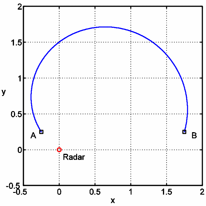
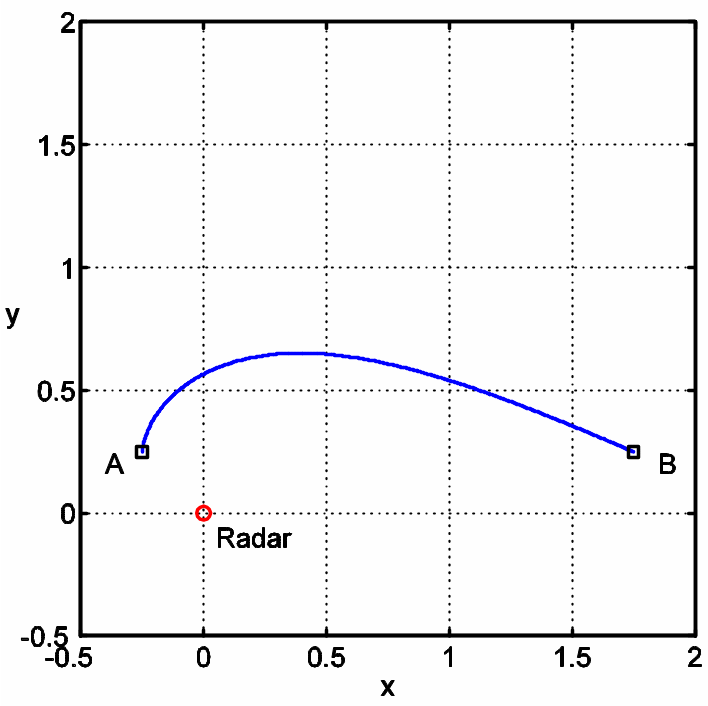
Figure 2. The flight path trajectory between the base (point A) and the mission objective (point B) with the enemy radar located at the origin for l=4.1994 The risk associated with this path is R=3.2208.

Figure 3, on the other hand, shows a separate solution path between points A and B where the trajectory length is shorter (l=2.2494). The risk associated with this path was found to be R=4.1283. The higher risk associated for this path is expected since the air vehicle is now travelling closer to the radar than the path shown in Figure 2. However, this value of risk appears to be lower than that reported in [3]. We discuss this discrepancy later.

Figure 3. The flight path trajectory between the base (point A) and the mission objective (point B) with the enemy radar located at the origin for l=2.2494. The risk associated with this flight path is R=4.1283.

By repeating the above steps for numerous values of trajectory lengths l between points A and B, we obtain Figure 4 which shows the relationship between the risk of detection, R, upon the trajectory length, l. We can see immediately that Figure 4 is exhibiting physically realistic behaviour—that is, as the flight path trajectory converges to the straight line from the base to the mission objective, one would expect the associated risk to increase dramatically. Using our numerical scheme the risk associated for path length l=2 (straight path from the base to the mission objective) is R=8.857. This value was also checked independently by calculating the risk directly from the risk expression Equation (4).

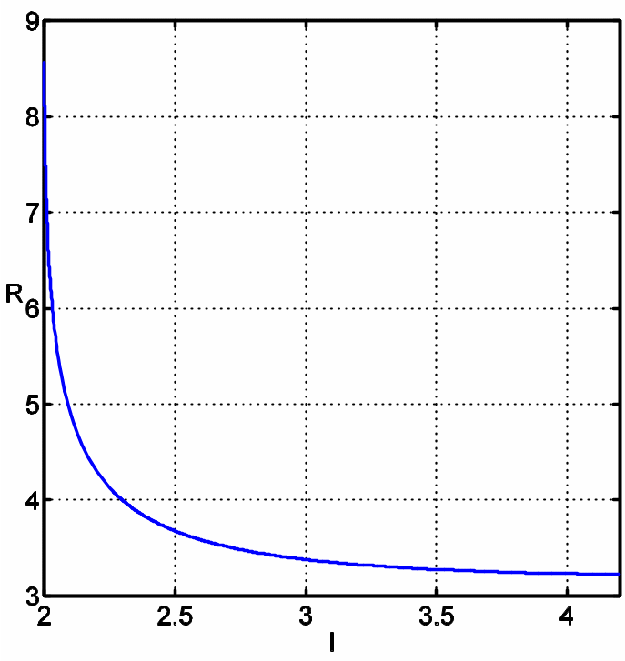
Figure 4. The dependence of the risk associated with enemy radar detection upon the trajectory length for the single radar problem. The locations of the base, mission objective and enemy radar are the same as those in Figures 2 and 3.

Furthermore, for l=3.2 we obtained a risk value of R=3.3256 which are precisely the values quoted in [3]. However, comparing Figure 4 with the corresponding plot in [3], it is clear that the risks computed here for various trajectory lengths are lower than those reported in [3] for the range 2 < l < 3.2 (noting that the risks evaluated at l=2 and l ≥ 3.2 appear to be the same with those reported in [3]). It is clear from Figure 4 that as the trajectory approaches the straight line path between points A and B, the risk increases exponentially. On the other hand, Zabarankin et al [3] reports a higher, but gentler increase in the risk for this range of l. We believe that the latter is most likely due to the discrete approximation to the flight path that these authors used in their study, and does not reflect the true risk associated with the flight path as calculated here.

Two enemy radars

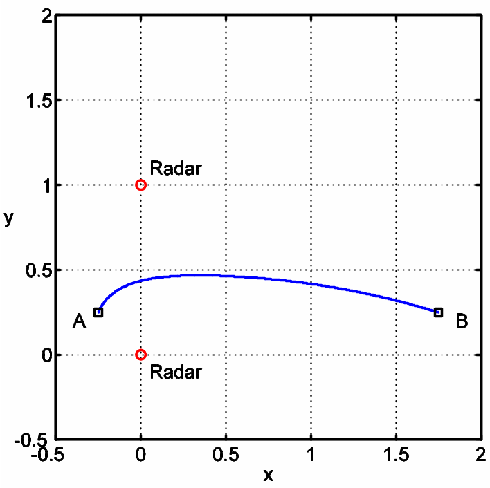
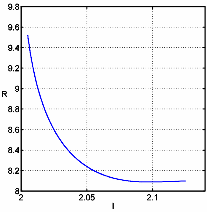
In this section we briefly present results for the case when the flight path is in a hostile environment with two enemy radars. Here we assume that the two radars are identical, that is, they have the same transmission power (although this assumption is not necessary for the numerical method used in this paper). We shall also assume that the locations of the base and the mission objective are the same as in the one radar problem discussed previously. As before, we shall assume that one of the radars is located at the origin (0,0), and investigate how the location of the other radar affects the flight path and the associated risk. Figure 5 shows the optimal path trajectory when the other radar is located at (0,1) for l=2.0974. The corresponding risk associated for the path shown in Figure 5 was found to be R=8.0878.

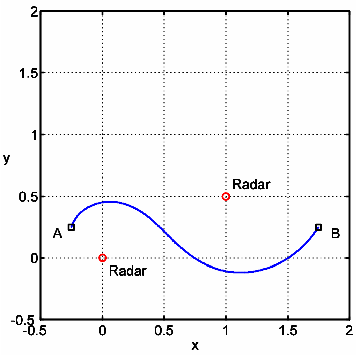
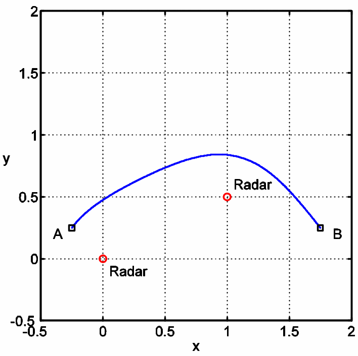
Figure 5. The flight path trajectory of length l=2.0974 between the base (A) and the mission objective (B) with two radars located at (0,0) and (0,1). The risk associated with the above path is R=8.0878.

For the case when the two radars are located in the positions shown in Figure 5, we can repeat the calculations for numerous values of l and determine the corresponding values of the risk associated with the flight path. Figure 6 shows how the risk depends upon the length of the trajectory for the above described case. Comparing Figures 4 and 6, it is clear that the risk has increased significantly with the inclusion of another radar. If we now change the location of the second radar from (0,1) to (1,0.5), then there is a possibility of having an “inner” trajectory (that is, a trajectory which goes between the two radars), and an “outer” trajectory (one that goes around the radars. Figures 7 and 8 show the “inner” and “outer” trajectories respectively from the base to the mission objective. In Figure 7 the “inner” trajectory length was found to be l=2.5186 with the associated risk of detection from the two radars as R=11.0861. For the case of the “outer” trajectory shown in Figure 8, the trajectory length was found to be l=2.5299 with the associated risk of detection from the two radars as R=11.7737.

Figure 6. The dependence of the risk R associated with two enemy radars located at (0,0) and (0,1) upon the trajectory length l.

Figure 7. ‘Inner’ trajectory from the base to the mission objective with two radars located at (0,0) and (1,0.5). The corresponding value of the risk for this path is R=11.0861.

Figure 8. ‘Outer’ trajectory from the base to the mission objective with two radars located at (0,0) and (1,0.5). The risk associated with the path shown in this figure is R=11.7737.

By repeated calculation of the trajectory lengths and the risk associated with each type of trajectory (“inner” and “outer”), one can plot a graph showing the risk as a function of trajectory length for both types of paths, as shown in Figure 9. Comparing the results for these different types of trajectories, it is clear that for shorter path length l, the “inner” trajectory path has less risk associated with it than the “outer” trajectory path. However, for longer path lengths, this difference becomes smaller, and for path lengths greater than approximately 2.6, the risk becomes lesser for the “outer” trajectories than for the “inner” trajectories. In fact, from our numerical investigations, the risk associated with the “inner” trajectories has a minimum of approximately 10.99 when the trajectory length l=2.84, whereas the risk associated with the “outer” trajectories reduces as the value of l increases.

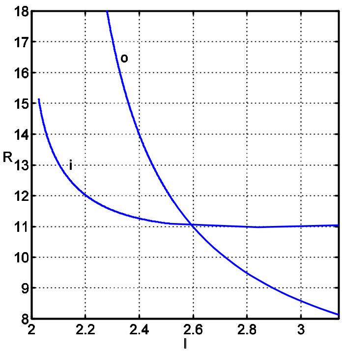
Figure 9. The dependence of the risk associated with two enemy radars located at (0,0) and (1,0.5) upon the trajectory length. The curve labelled ‘i’ represents solutions for the ‘inner’ trajectories (like those shown in Figure 7), whereas the curve labelled ‘o’ corresponds to solutions for the ‘outer’ trajectories, similar to those shown in Figure 8.

A common issue with optimization techniques is the question of finding the globally optimum solution. Many techniques locate locally optimum solutions (such as simulated annealing, [18]), with a number claiming to be able to find globally optimal solutions (some so-called ‘greedy’ heuristics [19]). Many problems are NP-complete (not solved in polynomial time) which means that there is no guarantee of finding the globally optimum solution, see [20]. Here, we find that the two trajectories shown in Figure 9 represent two locally optimum solutions with the ‘inner’ trajectory representing the Pareto-optimal set (see [21,22]) until the two trajectories intersect at approximately l = 2.6 whereupon the ‘outer’ trajectory becomes the Pareto-optimal set.

Conclusions

We have presented a method for determining the optimal path routes for a single air vehicle flying from its base to its mission objective when the flight is through an area consisting of enemy radar installations. Our method differs from the commonly used discrete optimization techniques in that it poses the problem in a continuous variable setting. It is clear that the method presented here does not suffer from problems associated with the gridding scheme utilized during discretization methods which can result in suboptimal paths. We have illustrated our method for two cases when the hostile environment consists of one and two radars. We believe that it would be feasible to extend the proposed method to obtain optimal paths through a threat environment consisting of a network of multiple radars, and even for the case of moving radars.

References

[1] R. Murphey, M. Zabarankin and S. Uryasev, “Trajectory Optimization in a Threat Environment”, Research Report 2003-9, ISE Dept, University of Florida, July 2003.

[2] J.L. Vian and J.R. More, “Trajectory Optimization with Risk Minimization for Military Aircraft”, AIAA, J. of Guidance, Control and Dynamics, Vol. 12, No. 3, pp. 311–317, 1989.

[3] M. Zabarankin, S. Uryasev, and P. Pardalos, “Optimal Risk Path Algorithms”, Cooperative Control and Optimization (R. Murphey and P. Pardalos Ed.), Kluwer Academic Publishers, Dordrecht, Vol. 66, pp. 271–303, 2002.

[4] J.J. Leary, Search for a Stealthy Flight Path Through a Hostile Radar Defense Network, Masters Thesis, Naval Postgraduate School, Monterey, CA, 1995.

[5] L.C. Thomas and J.N. Eagle, “Criteria and Approximate Methods for Path-Constrained Moving-Target Search Problems”, Naval Research Logistics, Vol. 42, pp. 27–38, 1995.

[6] M.C. Novy, Air Vehicle Optimal Trajectories for Minimization of Radar Exposure, Masters Thesis, Air Force Institute of Technology, Wright-Patterson Air Force Base, Ohio, 2001.

[7] J. Krozel and D. Andrisani II, “Navigation Path Planning for Autonomous Aircraft: Voronoi Diagram Approach”, AIAA, J. of Guidance, Control and Dynamics, Vol. 13, pp. 1152–1154, 1990.

[8] A. Meng, “Flight Path Planning Under Uncertainty for Robotic Air Vehicles”, IEEE National Aerospace and Electronics Conference, IEEE Press, pp. 359–366, May 1987.

[9] T.W. McLain and R.W. Beard, “Trajectory Planning for Coordinated Rendezvous of Unmanned Air Vehicles”, AIAA Guidance, Navigation and Control Conference, Paper no. AIAA-2000-4369, 2000.

[10] K.B. Judd and T.W. McLain, “Spline based Path Planning for Unmanned Air Vehicles”, AIAA Guidance, Navigation and Control Conference, paper no. AIAA-2001-4238, 2001.

[11] M.C. Selvestrel and S. Goss, “Optimal Flight Paths of Aircrafts: A Little Knowledge Goes a Long Way”, IEA/AIE Proceedings of the Eighth International Conference, pp 687–695, Gordon and Breach Science Publishers, 1995.

[12] S.A. Bortoff, “Path Planning for UAVs”, Proceedings of the American Control Conference, pp. 364–368, 2000

[13] M. Jun and R. D’Andrea, “Path Planning for Unmanned Aerial Vehicles in Uncertain and Adversarial Environments”, Cooperative Control: Models, Applications and Algorithms (S. Butenko, R. Murphey, and P. Pardalos Ed), Kluwer Academic Publishers, pp. 95–111, 2002.

[14] M. Norsell, “Multistage Trajectory Optimization with Radar-Range Constraints”, Journal of Aircraft, Vol. 42, No. 4, pp. 849–857, 2005.

[15] M. Norsell, “Radar Cross Section Constraints in Flight-Path Optimization”, Journal of Aircraft, Vol. 40, No. 2, pp. 412–415, 2003.

[16] M.I. Skolnik, Radar Handbook, New York: McGraw-Hill Book Company, Inc., 1990.

[17] Numerical Algorithms Group (NAG). http://www.nag.co.uk/

[18] E. Aarts and J. Korst, Simulated Annealing and Boltzmann Machines, John Wiley & Sons, New York, 1989.

[19] J. Seberry and J. Pieprzyk, Cryptography: An Introduction To Computer Security, Advances in Computer Science Series, Prentice Hall, New York, 1989.

[20] P.E. Black, “Greedy Algorithm”, in Dictionary of Algorithms and Data Structures [online], P.E. Black, ed., U.S. National Institute of Standards and Technology. 2 February 2005. (Accessed 16 June 2006). Available from http://www.nist.gov/dads/HTML/greedyalgo.html

[21] A.J.V. Skriver and K.A. Andersen, “A Label Correcting Approach For Solving Bicriterion Shortest-Path Problems” Computers & Operations Research, Vol. 27, No. 6, pp. 507–524, May 2000.

[22] N. Xiao, D.A. Bennett, and M.P. Armstrong, “Using Evolutionary Algorithms to Generate Alternatives for Multiobjective Site-Search Problems”, Environment and Planning, Vol. 34, pp. 639–656, 2004.

Authors

Harvinder Sidhu is a Senior Lecturer at the School of Physical, Environmental and Mathematical Sciences, University of New South Wales at the Australian Defence Force Academy. E-mail: h.sidhu@adfa.edu.au

Geoffry Mercer is a Senior Lecturer at the School of Physical, Environmental and Mathematical Sciences, University of New South Wales at the Australian Defence Force Academy. E-mail: g.mercer@adfa.edu.au

Mary J. Sexton has held various research positions within academia and the Australian federal government. miss_jane_maths@yahoo.com.au

Nadeem Ansari is a Research Assistant at the School of Physical, Environmental and Mathematical Sciences, University of New South Wales at the Australian Defence Force Academy. E-mail: n.ansari@adfa.edu.au

Zlatko Jovanoski is a Lecturer at the School of Physical, Environmental and Mathematical Sciences, University of New South Wales at the Australian Defence Force Academy. E-mail: z.jovanoski@adfa.edu.au