
Volume 9, Number 3, November 2006
The Vulnerability Of Laser Warning Systems Against Guided Weapons Based On Low-Power Lasers—Part III
- 1 Department of Aerospace, Power & Sensors, Cranfield University at the Defence Academy of the United Kingdom, Shrivenham, SN6 8LA.
Abstract
Theory for a laser sensor model was presented in Part I of this four-part series, followed in Part II by creation of a simulation employing MATLAB and Simulink. Verification of the laser sensor theory and simulation must be tested using experimentation and it is in this paper that construction and testing of the hardware necessary for this task is detailed.
Introduction
Theory for a laser sensor model was presented in Part I [1] of this four-part series, followed by creation of a simulation in Part II [2]. Verification of the laser sensor theory and simulation is to be tested using experimentation and it is in this paper that construction and testing of the hardware necessary for this task is detailed.
The value of any mathematical model rises significantly if its results can be validated using physical experimentation. For that purpose, an experiment mimicking the laser simulation was constructed and compared against theoretical results. Good correspondence was found between the theoretical and experimental results.
Experimental
The experimental setup was developed to verify the model is adequate as a physical description of laser sensor. The main aim of the setup was therefore to establish the signal to noise ratio of the sensor and determine the error displayed by the simulation.
The method essentially consisted of making successive measurements of the signal and noise levels output from the sensor at increasing distances from a laser source for differing levels of background illumination. These values are then compared to those determined from the model with the same operating parameters.
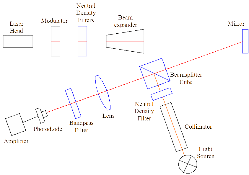
Figure 1 details the experimental setup. Three broad areas of layout correspond to the laser source, its propagation and addition to background illumination and the photo-sensitive device. Characteristics of elements in the experimental setup are given in Table 1. The laser source is a He-Ne-laser with the power of 1 mW modulated mechanically using an optical chopper. The optical pathway contains a neutral density filter in order to simulate power reduction at increased distances between the source and sensor. Also present were a beam-expander and beam-splitter with an additional light source to simulate gross distortion of the beam and the addition of background illumination. The sensor is a PIN-photodiode with a single cascade amplification stage. In order to be able to correctly use this experimental setup, it is necessary to calibrate the neutral density filters, the beam expander and the levels of background illumination with those that would be expected at differing ranges.
Mathematical model (without noise)
For simplification the experimental model is first developed in the absence of noise and then expended. Modifying the theory described in Part I [1], the experimental setup may be described mathematically using the following:
where:
Uamp—signal amplitude (volts).
Plas = 1 mW—continuous output power of laser source.
knf —transmission factor of neutral density filters.
kexp = 0.9—transmission factor of beam expander.
a = 25.4 mm—dimension of beamsplitter cube edge.
θ = 4.3 mrad—beam divergence in beam expander output.
Rcub = 191 cm—distance from a beamsplitter cube up to a receiving lens.
b = 15 mm—diameter of laser beam in beam expander output.
kcub = 0.5—transmission factor of beamsplitter cube.
D = 8 mm—diameter of receiving lens.
Ropt = 70 cm—distance from a beam expander to the beamsplitter cube.
kbf = 0.6—transmission factor of bandpass filter.
ελ = 0.4 A/W—spectral sensitivity of photodiode.
RF = 106 Ω—feedback resistance.
Signal amplitude measured at the photodiode is compared to the transmission of the neutral density filters. Dependence of the signal amplitude upon distance and any atmospheric effects may be described by:
where, Ta = 1 is the transmission factor of the atmosphere and R is the range to the laser source. Using this, it is then a relatively simple matter to calibrate the neutral density filters to represent the range and atmospheric transmission desired:
where Pin(R) is the expected power at the input of the photodiode and is given by:
Pin.exp is actual power at the input of the photodiode of the experimental setup for a given distance (R = 0.7 m) and can be calculated from Equation (4) as:
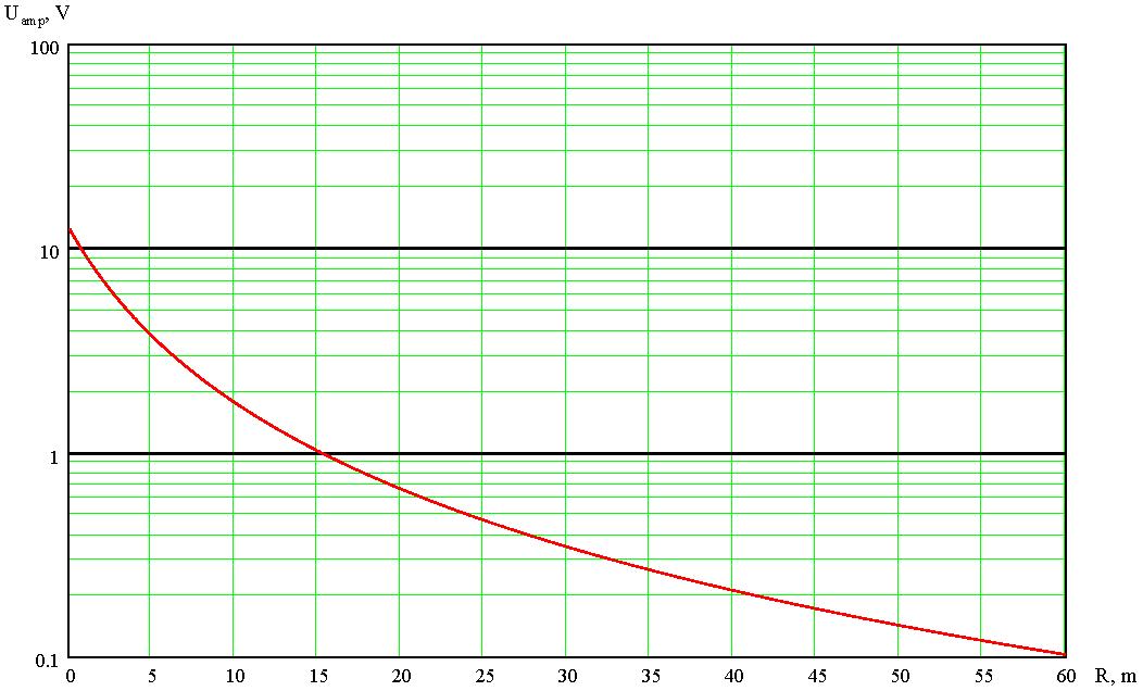
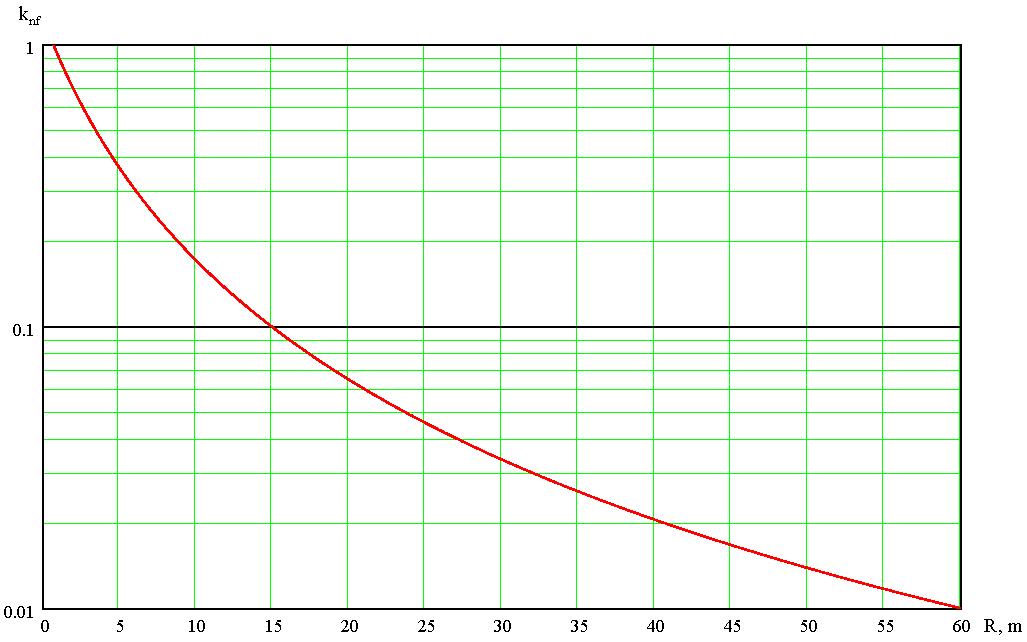
Figure 2, shows the amplifier output versus range and Figure 3, the calibration curve. Use of these curves permits the experimental setup to be used to simulate the gross effects of any signal attenuation due to atmospheric and range effects.
| Laser head | He-Ne Laser 1 mW | |
|---|---|---|
| Modulator | Pulse length—750 μs Pulse time—2700 μs | |
| Neutral density filters for signal | Variable | |
| Beam expander BE-10X | Beam divergence on output—4.3 mrad Output beam diameter - 15 mm Expansion—10× | |
| Mirror PF20-03-G01 | Ø 50.8 mm Reflectivity > 0.9 | |
| High intensity light source OSL1 | High output 150-W lamp | |
| Collimator OS6 | Light divergence on output— 33 mrad Ø output lens—50.8 mm | |
| Neutral density filters for background noise | Variable | |
| Beamsplitter cube BS014 | Size—25.4 mm Split ratio—50:50 | |
| Lens | Ø aperture—8 mm Focal length—40 mm | |
| Bandpass filter Ealing Corp. # 35-3904 | Transmission on 633 nm—0.6 Bandwidth FWHM—10 nm | |
| PIN Photodiode OSD1-5T | Sensitivity on 633 nm—0.4 A/W | |
| Amplifier | Feedback resistance—106 Ω |
| Generator | |
|---|---|
| Pulse period, s | 2700×10-6 |
| Pulse width, % | 27.778 |
| Pulse peak power, W | 0.686×10⁻³ |
| Atmosphere and optical system | |
| Diameter input lens, mm | 8 |
| Diameter output lens, mm | 25.4 |
| Divergence, mrad | 4.3 |
| Bandpass filter transmission | 0.6 |
| Noise | |
| Optical system loss factor | 0.5 |
| PD crystal diameter, mm | 1 |
| Spectral responsivity of PD, A/W | 0.4 |
| Input lens diameter, mm | 8 |
| Focal length, mm | 40 |
| Boltzmann constant, J·K-1 | 1.38×10⁻²³ |
| Temperature, K | 300 |
| Bandwidth, Hz | 20·103 |
| Load Resistance, Ω | 106 |
| Electron charge, Cl | 1.6×10⁻¹⁹ |
| Dark current, A | 0.5×10⁻⁹ |
| Photodiode | |
| Spectral responsivity of PD, A/W | 0.4 |
| Gain | 1 |
| Amplifier | |
| Feedback resistance, Ω | 106 |
| Bandwidth, Hz | 10.6×10³ |
| Gain | 1 |
| Comparator | |
| Spectral resposivity of PD, A/W | 0.4 |
| Feedback resistance, Ohm | 106 |
| Signal/Noise | 5 |
| Bandpass filter | |
| Transmission bandwidth on 0.5, μm | 0.628-0.638 |
The expected output voltage of the photodiode may now be estimated for a given transmission filter:
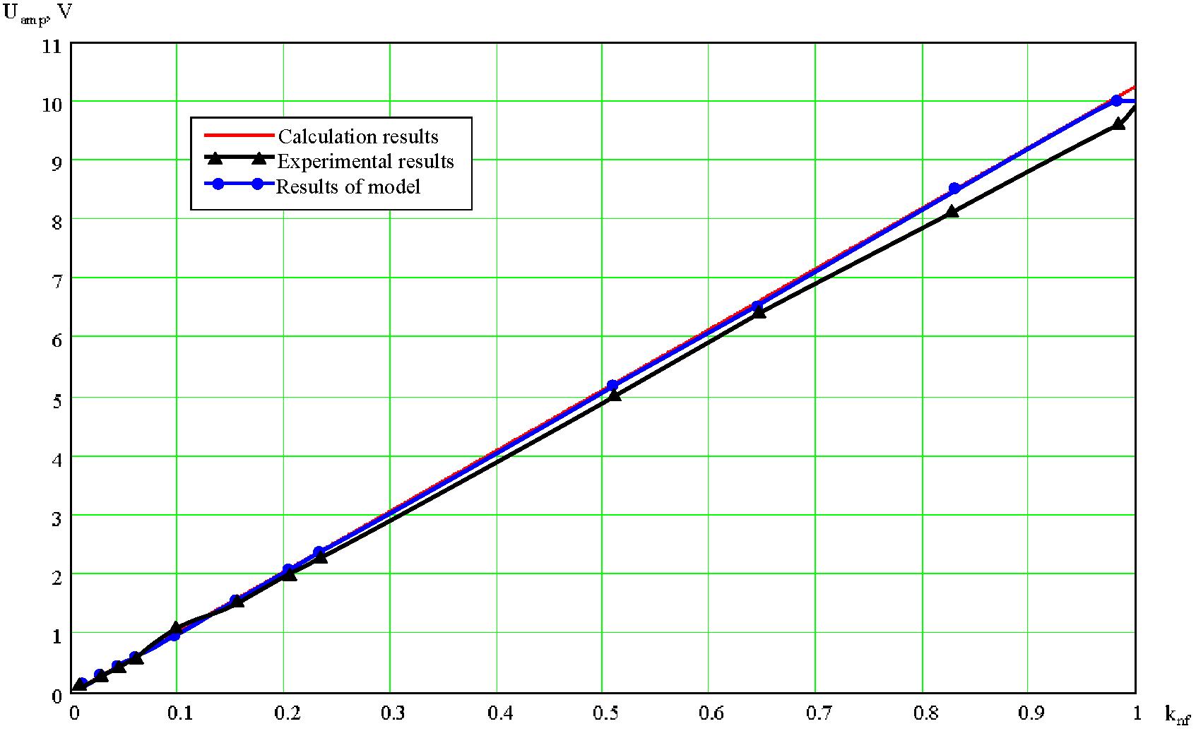
The signal amplitude output by the photodiode is measured with respect to the transmission filter density, with no additional background illumination in the first instance. This is then compared to values calculated using the simulation described in Part II. The parameters used to conduct the simulation are given in Table 2.
Figure 4 shows a graph comparing the results of the experimentation and simulation. Good correspondence between the developed model and the experimental results can be seen, though differences exist at higher signal levels. It is suggested that reasonable deviations may be explained by the non-linear operation of the cascade amplifier in the photodiode at high signal amplitudes
Mathematical model (including noise)
Expanding the experimental model to include a detailed estimation of the noise allows the effects on the photodiode to be evaluated and compared to the simulation. The main constituents of the noise include shot noise or dark current, caused by thermal generation of current free carriers, photon noise caused by statistical fluctuations of the optical signal, additional background illumination and finally electronic noise in any accompanying circuitry. Estimates of these noise constituents in the experimental setup when the amplifier has a narrow band (Δf=20 kHz) are low. This makes it difficult to determine experimentally.
For large values of background illumination, the measured voltage may be thought of as consisting of a constant component with an additional Gaussian distribution added to it. This causes the dynamic range of the photodiode to be reduced and, in some cases, the amplifier may be saturated leading to a total loss of signal. Saturation effects were simulated by adding an amplitude limiter to the model. The voltage of the limiter was set at 10 V in this case. In addition a noise constant was added to the input of photodiode. The noise constant is calculated:
where:
Uc—noise constant;
Pb—power of background;
ελ—spectral sensitivity of PD; and
RF—feedback resistance.
and:
where:
Pb—voltage due to background illumination;
B—background illumination;
Δλbf—optical filter bandpass;
kopt—transmission factor of receiving optical system; and
Tnf—transmission factor of neutral filter.
and:
where SD is the area of photodiode objective and finally:
where:
ω—the spatial angle of a field of view of the receiving device;
l—diameter of sensitive area of PD; and
f—focal length of photodiode objective lens.
Background illumination
A high intensity light source with output power of approx 150 W (T = 3 200K) is used to simulate background illumination with the following specifications:
- Wolfram Lamp;
- Pel = 150 W—electrical power;
- η=0.5—efficiency factor;
- l =3.0 cm—length of filament heater;
- r = 0.1 cm—radius of filament heater; and
- Δλ—spectral bandwidth.
The spectral radiant excitance of the source may be expressed in terms of power per unit area per unit solid angle per spectral unit:
where:
Popt=Pelη—optical output power of light source;
S=2πrl—lamp filament radiating surface area;
—the solid angle (for Lambertian radiators); and
—spectral range of the Light Source (0.4…2.4 µm).
The background illumination created in this manner is combined with the laser source via a beamsplitter. The level of background illumination is regulated using neutral density filters in an attempt to keep the spectral quality of the illumination constant throughout the experiment, rather than by adjusting the voltage supplied to the lamp. Measurements of the noise component and signal amplitude were made for differing levels of background illumination and field of view of the detector system. Care was taken so that the detector field of view did not exceed the beamsplitter’s output field.
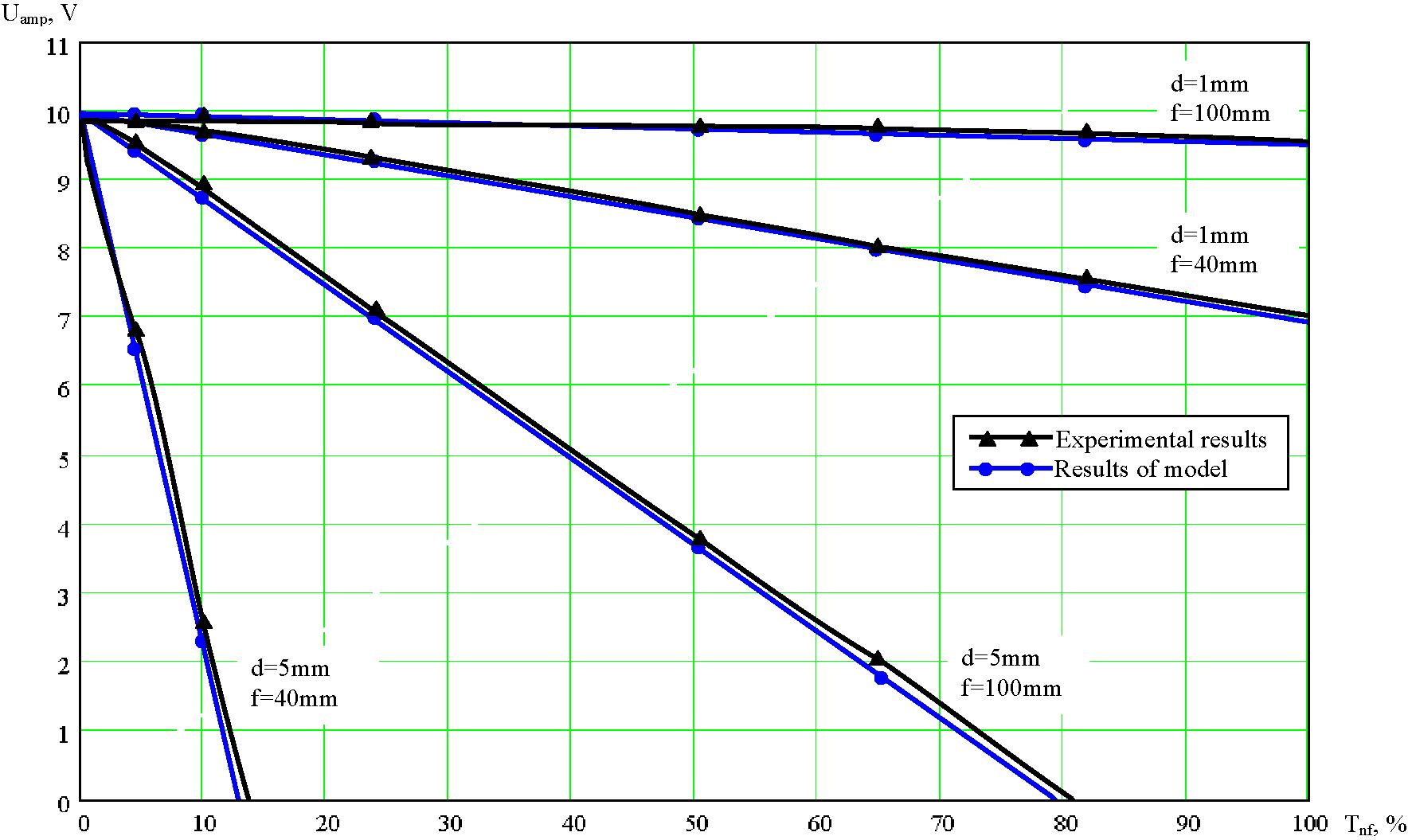
Two photodiodes were employed with active areas 1 mm and 5 mm diameter respectively. These were combined with two objectives of 40 mm and 100 mm focal length. Comparisons of experimental and simulated results were made at a variety of background illumination levels and simulated range. Figure 5 shows a summary plot of signal amplitude output from the photodiode circuitry versus background illumination filter transmission for constant range. It may be seen that there is good correspondence of the experimental and simulated results despite this variation in background noise, field of view and photodiode active area. Slight variations between the measured and actual results may be attributed to thermal noise, saturation effects in the photodiode and other sources of experimental noise.
Conclusion
Circuitry simulating the laser sensor simulation detailed in Parts I and II was built and tested against calculated results. The sensor circuitry and experimental arrangement was been designed such that it will simulate sources at varying range with the addition of background illumination to simulate the gross effects of scattering and absorption in the atmosphere. Comparisons between measured and modelled results for the laser sensor model show good correlation for differing photodiode active areas and objective focal lengths at varying range and noise levels.
References
[1] M. Al-Jaberi, M. Richardson, J. Coath, and R. Jenkin, “The Vulnerability of Laser Warning Systems Against Guided Weapons Based on Low-Power Lasers—Part I”, Journal of Battlefield Technology, Vol. 9, No. 1, March 2006.
[2] M. Al-Jaberi, M. Richardson, J. Coath, and R. Jenkin, “The Vulnerability of Laser Warning Systems Against Guided Weapons Based on Low-Power Lasers—Part II”, Journal of Battlefield Technology, Vol. 9, No. 2, July 2006.