
Volume 9, Number 2, July 2006
Sensitivity Analysis Of A Bayesian Belief Network In A Tactical Intelligence Application
- 1 Capability Analysis and Doctrine Branch, Army General Staff, PO Box 905, Trentham, Upper Hutt, New Zealand.
Abstract
In this paper, a variety of targeted sensitivity analysis approaches are explored for a Bayesian Belief Network (BBN) constructed as an expert tool for enemy course of action (COA) assessment at the tactical level in a conventional mid-intensity scenario. Robustness analysis is used to measure the level to which the posterior probability of the states at the root node are affected by instantiation of individual nodes in the network. Likewise, value of information analysis and gain in belief updating are used to compare how nodes of interest affect posterior probabilities at the root node, the former measuring Shannon Entropy and the latter Kullback Distance. Finally, sensor effectiveness analysis is used to measure how the reliability of reconnaissance and surveillance (R&S) assets affects updating of belief at the root node. It was found that each of the sensitivity analysis approaches could be used to optimise allocation of R&S, to identify the commander’s decision points, and to identify influential nodes for which the conditional probability tables (CPTs) should be refined. In terms of utility, it was concluded that, as in the case of the use of BBNs in the tactical COA assessment domain in general, the utility of sensitivity analysis of the BBN would be reduced in conditions of high operational tempo and myriad variables influencing tactical COA selection. Nevertheless, in a slower operational tempo environment, the benefits in refinement and utility of the BBN derived through sensitivity analysis would be significant.
Introduction
In a previous article [1], Bayesian Belief Networks (BBNs) were constructed to explore their use as expert tools to aid assessment of enemy course of action (COA) at the tactical level of war. Two scenarios were considered: Scenario 1, a conventional mid-intensity scenario; and Scenario 2, a Peace Support Operations (PSO) low-intensity scenario. Using intelligence collection plans for the respective scenarios, BNNs were constructed where enemy COA options that had been identified were root notes, and combat indicators and reconnaissance and surveillance (R&S) assets tasked to collect information on the combat indicators were child nodes separated from the root node by various generations depending on their relationship to the root node.
Sensitivity analysis can be used to refine such BBNs in a variety of ways. Because of the number of possible combinations of nodal states that could be involved in this process, simple sensitivity analysis can quickly become a significant task in terms of time and computational effort required. For this reason, it makes sense to target sensitivity analysis.
Using the Scenario 1 BBN from [1], the aim of this paper is to describe and comment on four forms of sensitivity analysis applied to a BBN designed to assess enemy COA at the tactical level:
- testing the robustness of a network,
- determining the value of information,
- calculating the gain in belief updating, and
- calculating sensor effectiveness.
Robustness analysis
Robustness analysis can be used to determine the extent to which posterior probabilities at the root node are changed when child nodes are instantiated. This type of robustness analysis is valuable in the context of using a BBN to assess enemy COA because it is important that the assessment is not heavily influenced by one or two nodes. If it were, there would be a potential for ‘nasty surprises’, that is, strong changes in the relative probabilities of the possible COAs after the inputting of just one or two pieces of evidence in the network. In such a case the commander would have very little warning of the need to alter an existing COA or activate a contingency plan. The ideal would be a gradual build-up of probability in one direction for each COA as evidence is added to the network. Robustness analysis can also be used to minimize affects of poorly calibrated or biased conditional probabilities elicited from experts. In that case, once influential nodes have been identified, their conditional probabilities can be refined using robustness analysis to gain an indication of the range in which changes in the conditional probabilities will change the posterior probabilities at the root node.
To perform robustness analysis, a prior probability distribution is compared with a posterior probability distribution after evidence has been added and propagated through the selected conditional probability distributions in the network. In a BBN, the posterior probability relates to a conditional probability as a quotient of two linear functions:
where: e is evidence,
x is the conditional probability, and
a,b,c and d are constants.
Netica, the programme used to construct the BBN, contains a facility for conducting single-finding sensitivity analysis. The report produced includes robustness measures in the form of the minimum and maximum values the posterior probability of a node will take when another node containing a conditional probability table is instantiated.
In terms of ranking, examination of the sensitivity report for the Scenario 1 BBN showed that COA2 tended to have the largest differences between prior and posterior probabilities. These ranged from 0.0205 to 0.4165. COA2 is therefore the least robust root node state to new evidence in the network. COA1 tended to be the next most sensitive, followed by COA3. Finally the posterior probabilities of COA4 tended to be the most robust to evidence propagated through the network, with differences between prior and posterior probabilities ranging from only 0.01038 to 0.11251. The exception to this was when evidence was instantiated at the aerial recon node tasked with detecting airmobile operation rehearsals. In that case the range between prior and posterior probabilities for COA4 was 0.3.
Although it is up to the expert to determine at what level a range of posterior probabilities becomes unacceptably high, the rankings of robustness are useful. In the context of combat intelligence, measures of robustness can be of value in alerting staff to the areas of greatest risk. In the analysis above, it can be seen that the enemy COA determined to be the most likely, namely COA3, is reasonably robust to new information, while COA4, determined to be the most dangerous COA, is the most robust, with the exception noted above. This is reassuring, in that what we assess are the most likely and the most dangerous COA the enemy could select are unlikely to become a reality out of the blue. The relative lack of robustness of COA1 and COA2, on the other hand, can be used to prioritise R&S tasking, in that those nodes to which COA1 and COA2 are least robust can be given a higher priority in the R&S collection plan in order to guard against unexpected changes in posterior probabilities making either COA1 or COA2 unexpectedly revealed as the course the enemy has chosen to pursue.
Robustness analysis of BBNs does not need to stop at assessing impact on the posterior probabilities of the root node, but rather can also be used to assess the impact on the decision that will be taken from the output at that root node. After all, combat intelligence is not an end in itself; rather its purpose is to provide information to the commander to support his or her decision-making. In view of this, the so-called threshold model for decision-making will be used to analyse robustness using the methodology developed by van der Gaag and Coupé [2]. This involves calculation of upper and lower bounds between which a belief network’s assessments can be varied without inducing a change in the recommended decision. The wider these bounds, the more robust the network and the decisions made based on it are deemed to be.
First, the decisions that would be made from the BBN network must be formulated. Using the Scenario 1 BBN as an example, it is assumed that if the BBN output supports COA1 or COA3, then the BG commander will not alter his own COA. However, if the BBN supports COA2 or COA4, then the commander will alter the COA. Thus, only outputs supporting COA2 or COA4 will require the commander to decide whether to alter his or her COA.
These decisions can be expressed as probability equations. The change COA threshold probabilities, P*(COA2) and P*(COA4), are the probabilities at which the commander is indifferent between maintaining the current COA or initiating an alternative COA. If the probability of an enemy COA, Pr(COA2) or Pr(COA4), exceeds the change COA threshold probability, that is Pr(COA2) > P*(COA2) or Pr(COA4) > P*(COA4), then the commander will decide to initiate a contingency plan. On the other hand, if Pr(COA2) ≤ P*(COA2) or Pr(COA4) ≤ P*(COA4), the commander will continue to follow the current COA.
It is also assumed that the BG commander is able to request further information from a higher HQ in the form of interpreted satellite imagery, to confirm what COA the enemy is pursuing. This introduces two further threshold probabilities. First, there is the maintain current COA—request satellite imagery threshold probability, P–(COA2) and P–(COA4), which is the probability threshold at which the commander is indifferent between the decision to maintain the current COA and the decision to request satellite imagery. Secondly, there is the satellite imagery—change COA threshold probability, P+(COA2) and P+(COA4), which is the probability at which the commander is indifferent between requesting satellite imagery and changing the COA straight away. The relationship between the various threshold probabilities is represented in Figure 1 for enemy COA2 and in Figure 2 for enemy COA4.


Taking enemy COA2 as an example, if the probability of COA2 exceeds the request satellite imagery—change COA threshold probability, that is if Pr(COA2) > P+(COA2), the commander will change his or her COA straight away. Otherwise, if P-(COA2) ≤ Pr(COA2) ≤ P+(COA2), the commander will request satellite imagery. After the evidence from that source has been added to the network, the commander will adopt an alternative COA only if Pr(COA2) > P*(COA2).
Related to threshold decision making is the question of the level of probability required to accept that a hypothesis node is in a certain state. The probability tells us how likely a certain COA is in relation to other possible COAs, but at what point does “more likely” become a sufficient measure upon which to act? In the context of Scenario 1, answering this question requires consideration of consequences or risks. For example, at what point does the risk of incurring unacceptable losses and failing to achieve the mission become so great as to force a decision to change the COA? For the purposes of this discussion, it will be assumed that the threshold probabilities take the following values.
| Description | Expression | Value |
|---|---|---|
| maintain current COA—request satellite imagery threshold probability | P–(COA2) | 0.20 |
| change COA threshold probability | P*(COA2) | 0.40 |
| request satellite imagery—change COA threshold probability | P+(COA2) | 0.55 |
| Description | Expression | Value |
|---|---|---|
| maintain current COA—request satellite imagery threshold probability | P–(COA4) | 0.05 |
| change COA threshold probability | P*(COA4) | 0.25 |
| request satellite imagery—change COA threshold probability | P+(COA4) | 0.45 |
Whereas the robustness analysis of network outputs performed above using Netica examined the movement of root node posterior probabilities for every conditional probability in the network, for robustness analysis within threshold decision making only the posterior probability shifts which result in a different decision are of interest. Robustness analysis for threshold decision making has to incorporate the various threshold probabilities quantified in Tables 1 and 2 above. Thus, now we are interested in calculating the range within which the networks outputs can be varied without inducing a change in decision.
Looking at COA2 only, the prior probability of this COA was 0.25. At that probability, we have P–(COA2) ≤ Pr(COA2) ≤ P+(CAO2). Thus, in the absence of any other information, the commander would request satellite imagery of enemy movements. If, once the satellite imagery evidence were entered into the network, the posterior probability of COA2 changed so that Pr(COA2) > P*(COA2), the commander would decide to initiate a new COA. However, assuming evidence had been entered into the BBN, the posterior probability ranges in the Netica sensitivity analysis report can be examined to discover which evidence updates belief in COA2 such that its posterior probability exceeds any of the relevant threshold probabilities. Resources could then be allocated to ensure that those variables which, when instantiated, caused the COA2 posterior probability to exceed P+(COA2), for example, had adequate R&S cover. That is, the R&S effort could be focused on collecting evidence from those variables to which decision thresholds were least robust. In that way, best effort could be made to avoid large and sudden changes in the posterior probabilities of COAs that could trigger a command decision.
Value of information
As was discussed above, a low robustness measure shows that a root node state is particularly sensitive to information from a particular node in the network. The flip side of this is that the node to which a root state is most sensitive will also be the most important node from which that root state can receive evidence. This introduces the concept of the value of information in the network.
Understanding the contribution of various nodes to the effectiveness of the network is valuable because resources are always scarce, and none more so than the R&S assets available to a tactical commander. Measuring the value of the information received from a particular asset can assist in deciding how to prioritise R&S allocation to derive the greatest effectiveness from the network.
The approach used to measuring the value of information will follow the methodology developed by Das [3]. The value of a piece of information from a node is considered to be the extent to which that piece of information reduces uncertainty at the root node. Current uncertainty equates to the prior probabilities of the various states at the root node. Uncertainty after evidence has been propagated equates to the posterior probability of root node states. Prior and posterior probabilities of states are compared using the following expression to give a measure, H(X), called Shannon Entropy:
where: X is a discrete random variable taking values {x1,…xn}, that is, the states of the root node,
P(X=xi) = P(xi) gives the probabilities of X.
Shannon Entropy measures “the average information required in addition to the current knowledge to specify a particular alternative” (p. 15) [3]. If we have complete knowledge about a state, then probability of that state will equal 1, which will correspond to zero entropy, H(X) = 0. If the current state of knowledge is total ignorance, then the entropy will be represented by a uniform distribution. “In general, therefore, H(X) provides a measure of the amount of information required to remove the ignorance expressed by the probability distribution P(xi)” (p. 15) [3]. H(X) can also be viewed as a measure of the spread of the probability distribution, P(xi). Although the propagation of new information in the network decreases uncertainty on average, for any particular instance it may increase uncertainty.
To separate the effects of prior probabilities from the effects of evidence propagation in the network, it is assumed that there is no prior knowledge of the root node, or hypothesis. All states are equally likely, thus maximising uncertainty. Figure 3 shows an excerpt of the Scenario 1 BBN with equally prior probabilities for the root node states.
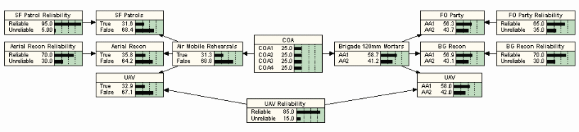
The uncertainty associated with this BBN is:
Now, nodes are instantiated as shown in Figure 4, representing the addition of new evidence into the network.
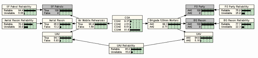
The uncertainty in the network after the addition of the new evidence is:
Thus, the change in Shannon Entropy is equal to the difference between uncertainty levels before and after the new evidence was added, namely 0.60200–0.28582=0.31618. This tells us that the evidence entered into the network in Figure 4 has reduced uncertainty by 0.31618 units. This process can be continued for individual nodes or for groups of nodes of interest throughout the network. For example, if UAV availability is reduced to one flight, then the entropy reduction associated with each use of the UAV to provide evidence in the network could be calculated in order to determine the priority of allocation.
In addition, value of information sensitivity analysis, along with robustness analysis, can be used to “reveal which parameters have a large effect on posterior probabilities, and, therefore, on which parameters the quantification effort should be focussed” (p. 223) [2].
Gain in belief updating
Another measure of the sensitivity of the network can be found by examining the gains or otherwise afforded by updating information. Given that it is rare for updating of a network to result in any one state of the root node having a posterior probability approaching 1, the distribution of posterior probabilities at the root node is important. As Das points out, “the form of P dictates our belief regarding the peculiarities of the situation being observed” (p. 19) [3]. He continues that “the sequence of probability distributions we obtain, as we go on updating information, should inform us how the situation is changing”.
The gain in belief updating is calculated by comparing root node posterior probabilities after updating (that is, the actual situation), P2, with the posterior probabilities had the updating not occurred (that is, the perceived situation), P1. This comparison can be expressed as follows:
The uncertainty of root node posterior probabilities with the updating is expressed as before:
Putting both of these expressions together we can measure the Kullback Distance between the two probability distributions, P1 and P2, denoted as D(P2||P1), which measures the worth of the updated information:
Das points out that the Kullback Distance is always positive, which can be interpreted as meaning that although new evidence may not reduce uncertainty in the network, it is always more efficient to update information.
An example of measuring the gain in belief updating can be shown using an excerpt from the Scenario 1 BBN. Suppose evidence was received from aerial reconnaissance and a UAV indicating the enemy were conducting airmobile rehearsals. This evidence would be updated through the network to update root node posterior probabilities as shown in Figure 5. The evidence indicates that the enemy is pursuing COA4, the airmobile operation to secure a bridge on AA1.
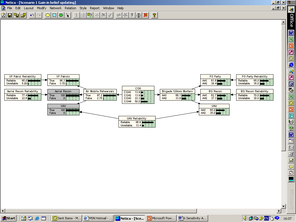
Suppose more evidence was received from an FO Party, a BG reconnaissance patrol, and a UAV, this time reporting that enemy brigade 120-mm mortars were observed moving along AA2. This is shown in Figure 6.
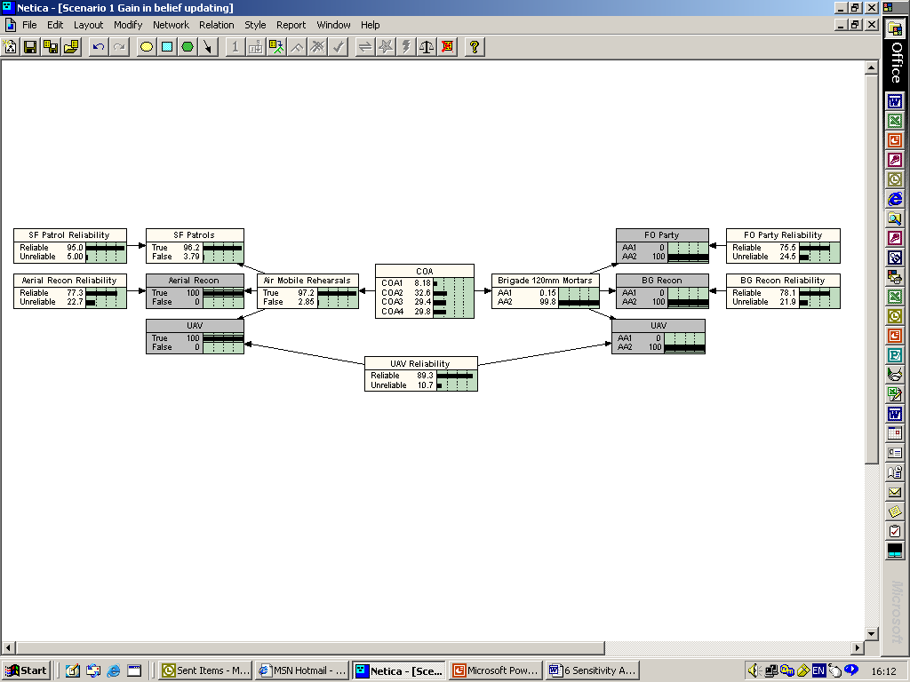
Table 3 compares the P1 and P2 distributions.
| x | COA1 | COA2 | COA3 | COA4 |
|---|---|---|---|---|
| P1(x) | 13.9 | 13.9 | 22.2 | 50.0 |
| P2(x) | 8.18 | 32.6 | 29.4 | 29.8 |
As can be seen, P1 indicated that COA4 was far more likely than the other enemy COAs. In addition, the peak in the distribution at COA4 indicated a low level of uncertainty in the distribution. However, the situation in P2 is quite different, with the distribution flattening out at COA2, COA3 and COA4, indicating an increase in uncertainty. Despite this, the gain in updating beliefs will be positive, because it is better to know the actual situation (P2) than to be misled by ones perception of a situation (P1). The gain from updating beliefs is calculated as follows:
While this figure of 0.0708 units of gain may not have much meaning in isolation, the Kullback Distance as a measure of the gain from updating beliefs can be applied to the Scenario 1 BBN to reveal the relative gain each R&S individual or group of R&S assets adds to the network. As in the case of measures of the value of information discussed above, the results of this analysis can be ranked and then used to determine R&S allocation priorities, so that assets are used where they will provide the most benefit to the network.
Sensor effectiveness
If the R&S assets in the BBNs were perfect, then if each sensor node were instantiated in state i, the indicator node it fed would also be in state i with a probability of 1. However, no sensor is perfect. This is acknowledged in the Scenario 1 BBN, where the element of unreliability in the sensor is fed into each R&S asset from its respective reliability node in accordance with the assigned conditional probability distribution. This point also brings us to the final form of sensitivity analysis to be applied, which facilitates the measurement of sensor effectiveness in a particular network. This measure tells us how the reliability of R&S assets affects the process of belief updating in a BBN.
The first step in the process is to define the concept of mutual information [8]. Given two random variables, X denoting the hypothesis variable, and Y denoting the indicator variable, the mutual information, I(X;Y), is defined as:
Das shows that:
and therefore:
I(X;Y) provides the average uncertainty reducing capacity of the random variable Y with respect to the uncertainties in X.
A third random variable, Z, can be introduced to denote the sensor which provides information to Y. The uncertainty reducing capacity of Z with respect to uncertainties in X can now also be denoted as:
and again it follows that:
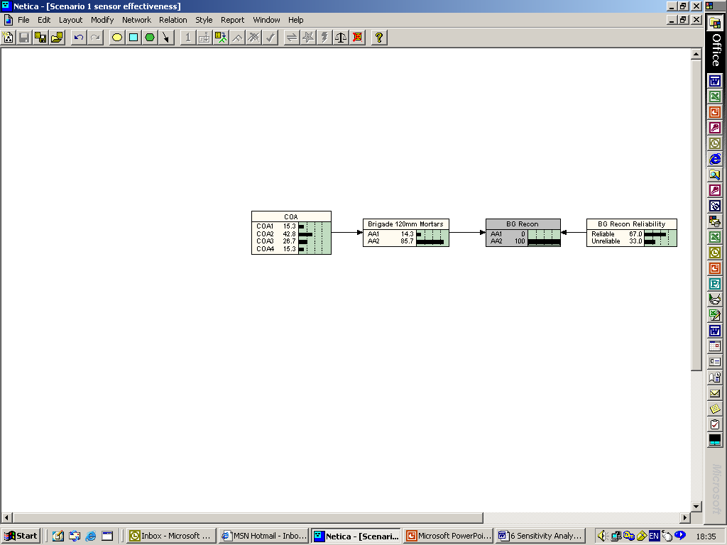
To provide a yardstick against which to compare posterior probabilities updated by evidence from Z, the hypothesis variable, X, must have prior probabilities which reflect maximum uncertainty. This starting point is depicted for an excerpt of the Scenario 1 BBN in Figure 7, where the COA node states have been given maximum uncertainty prior probabilities in the form of equal prior probability for each state. In Figure 7 the random variable X is the COA hypothesis node; the random variable Y is the Brigade 120mm Mortars indicator node; and the random variable Z is the BG Recon sensor node.
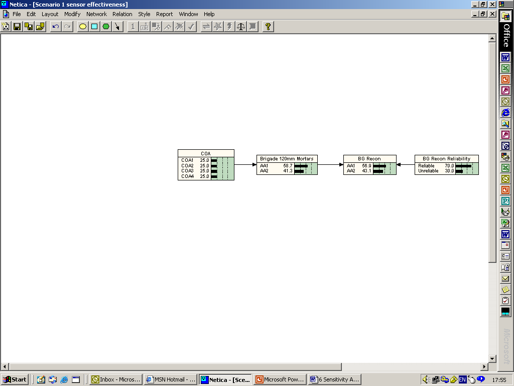
Table 4 lists the posterior probabilities of the nodes.
| Probability Distribution | Node States | |||
|---|---|---|---|---|
| P(x) | COA1 | COA2 | COA3 | COA4 |
| 0.25 | 0.25 | 0.25 | 0.25 | |
| P(y) | AA1 | AA2 | ||
| 0.587 | 0.413 | |||
| P(z) | AA1 | AA2 | ||
| 0.569 | 0.431 |
In order to calculate I(X;Y) we need values for H(X|Y) and H(X|Z). H(X|Y) is obtained by instantiating Y in its various states, as in Figures 8(a) and (b). Table 5 shows the values of P(x|y):
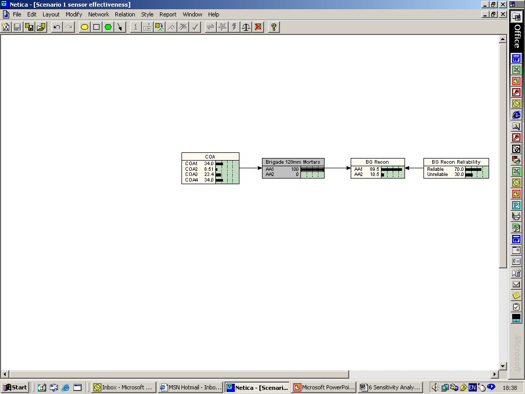
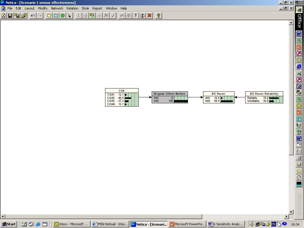
| X | |||||
|---|---|---|---|---|---|
| COA1 | COA2 | COA3 | COA4 | ||
| Y | AA1 | 0.3400 | 0.0851 | 0.234 | 0.3400 |
| AA2 | 0.121 | 0.485 | 0.273 | 0.121 |
H(X|Z) is obtained by instantiating Z in its various states, as shown in Figures 9(a) and (b). Table 6 shows the values of P(x|z):
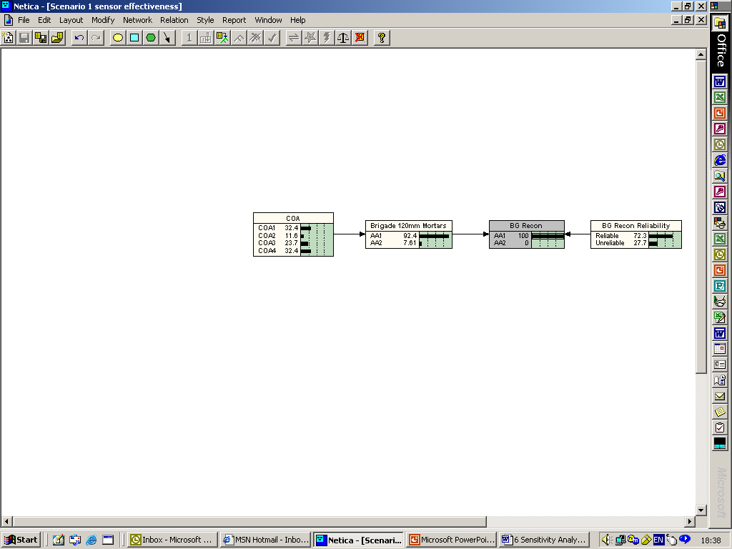
| X | |||||
|---|---|---|---|---|---|
| COA1 | COA2 | COA3 | COA4 | ||
| Z | AA1 | 0.324 | 0.116 | 0.237 | 0.324 |
| AA2 | 0.153 | 0.428 | 0.267 | 0.153 |
This information can now be drawn together to calculate the effectiveness of BG Recon in this branch of the network. It was stated above that:
and:
Reading from Table 4, H(X) can again be calculated:
H(X|Y) can also be calculated for all states of Y from Table 5 as follows:
(17)
Similarly, H(X|Z) can be calculated for all states of Z from Table 6:
(18)
Thus:
so:
This result tells us that the uncertainty reducing capacity of the BG Recon nodes under consideration differs from an ideal sensor by 0.0226 units. Again, the same calculation can be carried out for other sensors to determine which is most effective in reducing uncertainty in order to prioritise allocation of scarce R&S resources.
Conclusion
All four of the targeted sensitivity analysis approaches examined measured the sensitivity of posterior probabilities at the COA node, but each approach did so by different means. First, robustness analysis was applied to the Scenario 1 BBN as method of shielding the commander against large swings in posterior probabilities at the COA node when evidence is propagated through the network. The robustness of the various states at the root node to new evidence was calculated for each child node in the BBN. In this case it was found the most robust COA were the most likely and the most dangerous, which is reassuring in the tactical enemy COA assessment context. The exception to this, namely that despite being the most robust overall COA4 was actually very sensitive to a particular piece of information, could then be used to prioritise R&S assets to shield against that lack of robustness and the combat indicator concerned could become a decision point for the commander. Robustness analysis was extended and applied to threshold decision making to assist the commander in understanding which nodes would provide evidence that would constitute a decision point. To do this, threshold probabilities were developed and then only shifts in posterior probabilities that crossed the thresholds were of interest to the commander. Again, resources could be allocated to those nodes producing the shifts in posterior probabilities of interest, and those thresholds could become decision points in the commander’s planning, although critical to this process would the correct assessment of meaningful levels for probability thresholds in the first place.
The second form of sensitivity analysis explored was value of information. This approach revealed the effectiveness of each of the nodes in the network, that is, the extent to which a piece of information reduces uncertainty at the root node. This was achieved using the measure of Shannon Entropy to compare root node prior and posterior probabilities with respect to evidence for all the nodes of interest in the network. The resulting Shannon Entropy measures could be used to optimise R&S asset allocation (by identifying which nodes are best at reducing uncertainty at the root node) and to focus refinement of conditional probability tables (CPTs) developed to quantify the network. Similarly, gain in belief updating, the third approach explored, compared prior and posterior probabilities at the root node as evidence was propagated, but this time by measuring the Kullback Distance between the prior and posterior probability distributions. Kullback Distances could be calculated for all nodes in the network and, again, be used to allocate R&S assets or to refine CPTs for those nodes that produce the biggest gains in belief updating. Finally, sensor effectiveness analysis was used to measure how the reliability of R&S assets affects the updating of posterior probabilities in the root node.
For all the forms of sensitivity analysis discussed here, calculations must be made for all the nodes of interest in the network in order to make comparisons. This could be a time-consuming process, although Netica, the BBN programme, used to construct the BBN for this paper, does have a sensitivity analysis tool. As all the approaches examined here essentially deal with the relationship between root node prior and posterior probabilities with respect to specific nodes or groups of nodes, it may well be that a sensitivity analysis tool such as contained in Netica is sufficient for the purpose of optimizing R&S asset allocation and refining the CPTs of influential nodes. However, the more targeted the analysis needs to be, the more unlikely it is that a generic sensitivity analysis tool would suffice.
The earlier paper describing the construction of the BBN used here also discussed the utility of BBNs in the tactical enemy COA assessment domain and concluded that there are a number of problems associated with this domain [1]. This is especially the case where the tempo of operations and the number of variables involved in COA selection at the tactical level makes the modification of the quantification of the network both necessary and yet difficult to complete in a timely or expert manner. For the same reasons, sensitivity analysis of a BBN in such a situation would also be both more necessary and yet more difficult to complete in a timely or expert manner. Nevertheless, in a tactical situation with a slower operational tempo, such as may be the case in a PSO environment, sensitivity analysis would make the BBN more robust through the refinement of the CPTs of influential variables, and at the same time could enhance R&S resource allocation decisions and identification of decision points for the commander. Naturally, the same would apply to a BBN used as an indicator and warning tool at the tactical level, although the generic nature of such BBNs, as discussed in the earlier paper, would reduce the specificity of the network in the first place, so sensitivity analysis would likely not yield as much value as in the case of a more specific network.
References
[1] A.J. Brosnan, “”Use of Bayesian Belief Networks for Enemy Course of Action Assessment at the Tactical Level”, Journal of Battlefield Technology, Vol. 9, No. 1, pp. 31–40. March 2006.
[2] V.M. Coupé and L.C. van der Gaag, “Properties of Sensitivity Analysis of Bayesian Belief Networks”, Annals of Mathematics and Artificial Intelligence, Vol. 36, pp. 323–356, 2002.
[3] B. Das, Representing Uncertainties Using Bayesian Networks, DSTO-TR-0918, DSTO, Australia, 1999.