
Volume 9, Number 2, July 2006
The Vulnerability Of Laser Warning Systems Against Guided Weapons Based On Low-Power Lasers—Part II
- 1 Department of Aerospace, Power & Sensors, Cranfield University at the Defence Academy of the United Kingdom, Shrivenham, SN6 8LA.
Abstract
Laser-assisted weapons, such as laser-guided bombs, laser-guided missiles and laser-beamriding missiles pose a significant threat to military assets in the modern battlefield. Laser-beamriding missiles are particularly hard to detect because they use low-power lasers. They are even harder to defeat because current countermeasures are not designed to work against this threat [1]. The aim of this project is to examine the vulnerability of laser-warning systems to guided weapons, to build an evaluation tool for laser-warning receivers (LWRs) and seekers, and to identify suitable countermeasures for laser-beamriding missiles that use low-power lasers in their guidance systems. The project arose because of the unexpected results obtained from extensive field trials carried out on various LWRs in the United Arab Emirates desert, where severe weather conditions may be experienced. In order to approach the subject, a computer model has been developed to enable the assessment of all phases of a laser-warning receiver and missile seeker. MATLAB & SIMULINK software have been used to build the model. During this process experimentation and field trials have been carried out to verify the reliability of the model. This project enables both the evaluation and design of any generic laser-warning receiver or missile seeker and specific systems if various parameters are known. Moreover, this model will be used as a guide to the development of reliable countermeasures for laser-beamriding missiles. Part I of this series outlined the theory required to construct a computer model for a laser-beamriding missile engagement. This second part presents the implementation of the model using MATLAB and Simulink, the inputs required of the model, and the outputs generated. These results are analysed to determine the correct functionality of the model prior to its verification with laboratory-based experimental results and full-scale field trials (as presented in Part III).
Introduction
The model is written as a combination of Simulink blocks and Matlab code in a modular fashion. The basic methodology, as reported in Part I of this series of papers, depicts the whole system from the laser source where the signal is generated, through to the receiver which represents the laser-warning receiver and/or the laser-missile seeker.
Laser detection sensor model
The laser-detection-sensor model has been developed on the basis of the mathematical equations described in Part I of this series of papers [1]. The model is composed of a set of subsystem blocks (see Figure 1) incorporating an algorithm representing the functionality of that block in the laser-detection-sensor process.
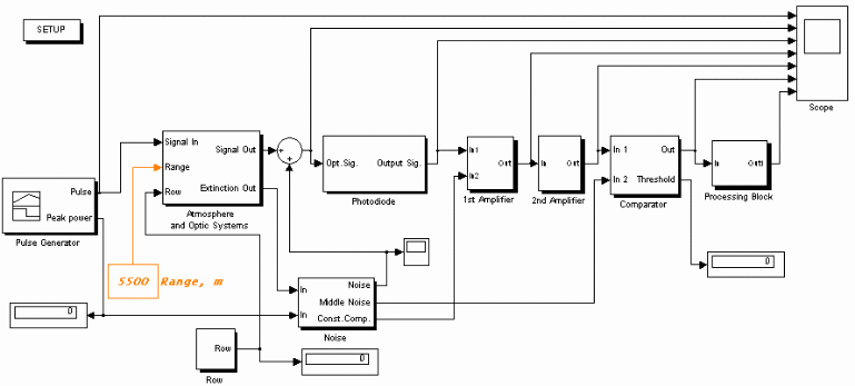
Each block has an input panel to insert and correct the initial parameters to realize the internal mathematical transformations of the algorithm and also investigate its functionalities. The model also provides an opportunity for visualization of all the output signals of each block with help of the in-built oscilloscope. The result of the model is fixed as a header: “DETECTED” or “NOT DETECTED”.
The structure of model includes the following blocks:
- Pulse Generator.
- Atmosphere and Optic System.
- Row.
- Noise.
- Photodiode.
- 1st Amplifier. and 2nd Amplifier.
- Comparator.
- Processing Block.
- Setup.
- Range.
- Scope.
The block “Pulse Generator” represents the subsystem modelling the formation of the laser signal as a Gaussian Pulse of the required duration and amplitude, and also the periodicity of the pulses with the set duration and the period of recurrence. The given subsystem is realized on the basis of standard elementary blocks from the Simulink library. The internal clock forms the continuous modelling time and this reference is adhered to from the start of the model.
The block “Atmosphere and Optic System” represents the subsystem modelling the effect of attenuation and distortion of the laser radiation at it passes through a turbulent atmosphere and the optical channel. Once again the subsystem is realized on the basis of standard elementary blocks of Simulink library and uses data derived from the off-line running of the LOWTRAN VII atmospheric computer code [2] and the appropriate value is selected by the block “Row”.
The “Noise” block represents the subsystem in which the noise signal is formed resulting in an input for the photodetector. This consists of the shot noise and dark current of the photodetector, the shot noise of the background radiation, and thermal noise of the electronics.
The “Photodiode” block represents the subsystem in which the transformation of the optical signal to the electric signal is carried out.
The “1st Amplifier” subsystem carries out the transformation of the photodiode output current pulses to pulses of voltage and amplifies the signals up to the required value. In the model it is realised as consecutive switching on/off of the block of the ideal amplifier, the higher frequency filter, and the peak terminator (which simulates the process of saturation of the amplifier).
The “2nd Amplifier” subsystem is working as an ideal amplifier with a fixed gain and the limited bandpass. It is again realized as consecutive switching on/off of the block of the ideal amplifier, the low frequency filter and the block of the peak terminator modelling the process of saturation in the intensifying cascade. The bandwidth of the intensifying cascade has been chosen from the value of the width of laser signal. The gain of amplification has been designed on the basis of satisfying the condition of maintaining the required size of signal amplitude for confident operation of the comparator.
The “Comparator” block represents the subsystem that forms an output pulse only in the case of the input signal amplitude exceeding a threshold level. It has two inputs, one is the useful signal, and the other is the threshold voltage. In the circuit of threshold voltage formation, there is a block to input the value of the signal/noise ratio that provides the required value to achieve the correct detection probability and false-alarm rate.
The “Processing Block” depicts the logic functions of either the LWR or the laser seeker and may incorporate pulse counting, matched filtering, and so on.
The “Setup” block represents Graphical User Interface which opens dialog windows for the input and corrections of the initial data.
The “Range” block is intended for the input of values of the distance from the source of the laser radiation to laser sensor.
The “Scope” block enables the visual display of the signals which are generated by each of the separate model elements.
Graphical user interface (gui)
A GUI has been designed in Matlab to facilitate the easy running of the model. Figure 2 shows the GUI layout.
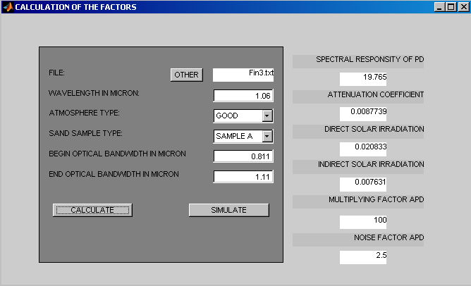
It is clear from the figure that the user has the capability to change the source file by clicking on the “OTHER” button which opens the files folder containing the input data.
The GUI contains the following inputs:
- Wavelength. The user enters the wavelength (in µm) of the threat laser.
- Atmosphere type. The user has an option to select the weather condition from five possibilities.
- Sand samples. As mentioned before we are using three sand samples from the United Arab Emirates desert and here the user has an option to choose one of them.
- Begin optical bandwidth. The lower wavelength limit (in µm) of the complete optical system (including any filters).
- End optical bandwidth. The upper wavelength limit (in µm) of the optical system (including any filters).
After inputting this initial data the “Calculate” button is clicked. This then calculates the following data (for input into the appropriate Simulink block):
- Spectral responsivity of the photodiode.
- Attenuation coefficient.
- Direct solar irradiation.
- Indirect solar irradiation.
- Multiplying factor of APD.
- Noise factor of APD.
After this the model is run by clicking the “Simulate” button.
Atmospheric data
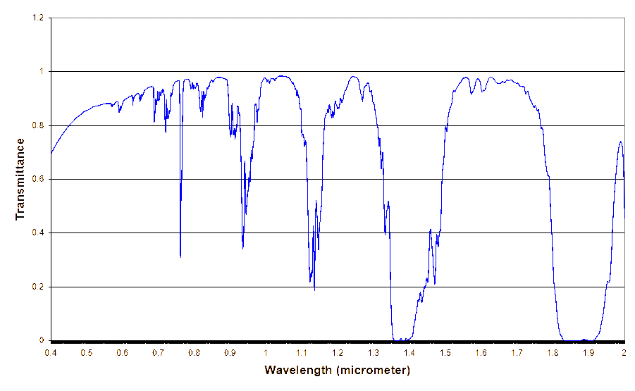
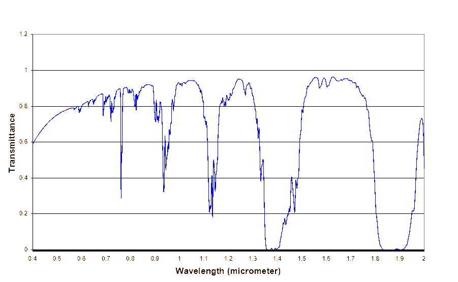
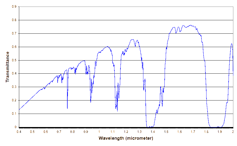
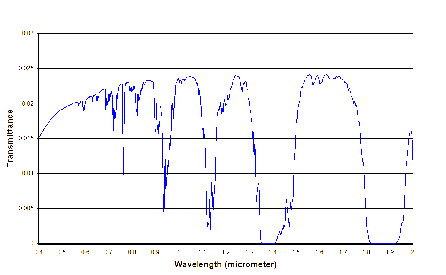
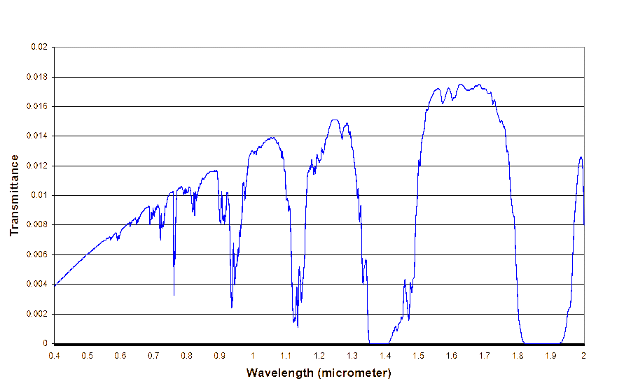
The choice of the atmosphere type used is based on information on the current weather conditions. The following five weather types have been modelled: Good, Typical-I, Typical-II, Bad-I, and Bad-II. These conditions are related to the type of weather typical in the UAE during the four seasons of the year. The attenuation of the laser radiation for different weather conditions is calculated with the LOWTRAN VII atmospheric computer code. This can be seen in Figures 3 to 7.
Sand data
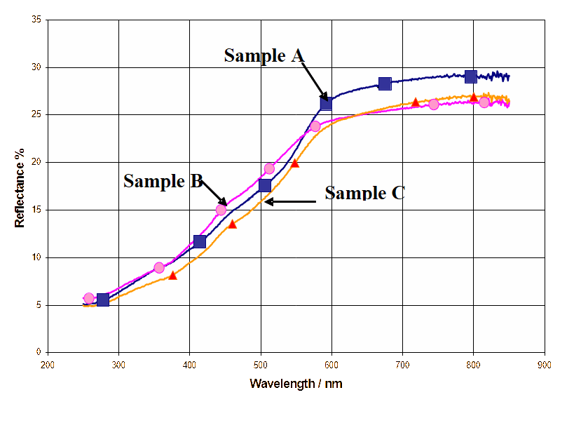
The choice of the background sand type as a reflecting surface is carried out on the basis of the information on the location of laser sensor and results of measurements of the reflection of various samples of UAE sand. Results have shown there to be three basic types (A, B, and C) of sand and their measured values are shown in Figure 8.
Photodiode data
The detector is an essential component for our system and is one of the crucial elements which dictate the overall system performance. Its function is to convert the received optical signal into an electrical signal, which is then amplified before further processing.
Therefore when considering signal attenuation along the path, the system performance is determined at the detector. The following criteria define the important performance and compatibility requirements for detectors [3]:
- High sensitivity at the operating wavelength. The quantum efficiency should be high to produce a maximum electrical signal for a given amount of optical power.
- High fidelity. To faithfully reproduce the received signal waveform electrically.
- Short response time to obtain a suitable bandwidth.
- Minimum noise. Typically the lower the dark current the better is the detector.
- High internal gain with low noise circuitry.
- High reliability. Capable of continuous stable operation for many years.
- Relatively low cost.
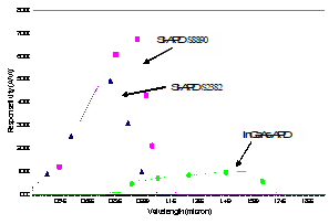
From the above and the requirement for as long a range detection as possible (see Part I of this series of papers [1]), APDs are chosen as the most appropriate detector. Three Photodiodes have been chosen to cover the wavelength of interest (typically 0.4–1.7 μm) [4]:
- Si APD S2382 (Hamamatsu); maximum spectral response at λmax=0.8 µm.
- Si APD S8890 (Hamamatsu); maximum spectral response at λmax=0.94 µm.
- InGaAs APD C30644E (EG*G); maximum spectral response at λmax=1.55 µm.
Figure 9 shows the responsivity (spectral response) of these three APDs.
In the model an automatic selection criteria for the photodiode has been implemented depending on the laser source wavelength. The spectral coverage of each choice is as defined below:
- Δλ1=0.4…0.81 µm—Si APD S2382
- Δλ2=0.811…1.11 µm—Si APD S8890
- Δλ3=1.111…1.7 µm—InGaAs APD C30644E
The model also contains values for the gain or Multiplying Factor (М) and Noise Factor (X) for the APDs. Typical values are М=100, X=2.5.
Other data
Other inputs (direct solar irradiance, indirect solar irradiance as discussed in Part I [1]) are called by the MATLAB code. A typical set of input data can be seen in Table 1.
Model functionality testing
Runs with the model have been conducted with various weather conditions and atmosphere turbulence levels and also for various values of devices parameters. Figure 10 shows the oscilloscope output signals for various model blocks for the initial data of Table 1 and a range of 5,500 m to the laser source.
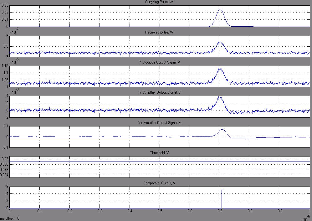
The comparative analysis of the amplitudes of useful signal and noise on the oscilloscope shows that the model is functioning as expected.
The results of the maximum detection range of the laser source under various atmospheric conditions and various spectral ranges are given in Table 2. These are simply accomplished by running the model for successive increases in range until threshold detection is not achieved.
The results of the maximum detection range of the laser source (λ=1.06 μm) under various atmospheric conditions and various background sand types are given in Table 3.
Conclusion
A laser-sensor model has been built and tested for different cases and weather conditions. The outputs of the model demonstrate it is behaving as predicted. The model is flexible and general enough to encompass all expected variations and can easily be updated with new or different data files.
Part III of this series will compare the model outputs to the results of a series of laboratory-based experiments and the results from some full-scale field trials, with real laser-beamriding systems and laser-warning receiver systems, in the UAE. This will demonstrate the validity of the model as an accurate predictor of the laser-beamrider engagement. This will engender a high degree of confidence in Part IV, the last of this series, which will study the various factors that influence the overall performance of the laser sensor, will formulate recommendations on the optimization of the various parameters and will hence enable realistic predictions for optimisation of LWRs and countermeasure analysis to be carried out.
| APD type | λ μm | ∆λ μm | Maximum Range (km) | ||||
|---|---|---|---|---|---|---|---|
| Good | Typ-I | Typ-II | Bad-I | Bad-II | |||
| Si APD S2382 | 0.63 | 0.4– 0.81 | 4.3 | 4.1 | 3.0 | 2.1 | 1.9 |
| Si APD S8890 | 1.06 | 0.81– 1.11 | 5.5 | 5.3 | 4.2 | 2.2 | 2.1 |
| InGaAs APD C30644E | 1.54 | 1.11– 1.7 | 7.2 | 7.1 | 5.7 | 2.5 | 2.4 |
| Setup | |
|---|---|
| Wavelength in microns | 1.06 |
| Atmosphere type | Good |
| Sand sample type | Sample A |
| Begin optical bandwidth, µm | 0.811 |
| End optical bandwidth, µm | 1.11 |
| Generator | |
| Gauss pulse mean, s | 35×10-9 |
| Gauss pulse standard deviation, s | 13×10-9 |
| Pulse peak power, W | 25×10-3 |
| Atmosphere and optical system | |
| Absorption coefficient | From LOWTRAN |
| Dispersion coefficient | From LOWTRAN |
| Diameter input lens, mm | 30 |
| Diameter output lens, mm | 30 |
| Divergence, mrad | 3 |
| Squared structural constant of refraction coefficient, m-2/3 | 52×10-17 |
| Noise | |
| Optical system loss factor | 0.5 |
| PD crystal diameter, mm | 0.5 |
| Input optic lens diameter, mm | 30 |
| Focal distance, mm | 40 |
| Boltzmann constant, J·K-1 | 1.38×10⁻²³ |
| Temperature, K | 328 |
| Bandwidth, Hz | 33×106 |
| Load resistance, Ω | 105 |
| Electron charge, Cl | 1.6×10⁻¹⁹ |
| Dark current, A | 0.5×10⁻⁹ |
| Background noise | |
| Coefficient distribution of brightness | 0.172 |
| Angle between sun and optical axis, degrees | 40 |
| Dispersion coefficient of clouds | 0.001 |
| Spectral brightness of night sky, W/cm2·μm·srad | 10·10-10 |
| Photodiode | |
| Spectral sensitivity, A/W | From Lookup Table |
| 1st Amplifier | |
| Gain | 4 |
| Derivator characteristic time, s | 900×10-9 |
| Internal resistance, Ω | 103 |
| 2nd Amplifier | |
| Gain | 20 |
| Bandpass edge frequency, Hz | 30×106 |
| Comparator | |
| Integrator characteristic time, s | 100×10-9 |
| Tuning coefficient | 1 |
| Sand type | Maximum Range (km) | ||||
|---|---|---|---|---|---|
| Good | Typ-I | Typ-II | Bad-I | Bad-II | |
| A | 5.5 | 5.3 | 4.2 | 2.2 | 2.1 |
| B | 5.9 | 5.7 | 4.4 | 2.2 | 2.1 |
| C | 5.8 | 5.6 | 4.3 | 2.2 | 2.1 |
References
[1] M. Al-Jaberi, M. Richardson, J. Coath, and R. Jenkin, “The Vulnerability of Laser Warning Systems Against Guided Weapons Based on Low-Power Lasers—Part I”, Journal of Battlefield technology, Vol. 9, No. 1, March 2006.
[2] Lowtran 7 atmospheric code, available through Ontar Corporation, http://www.ontar.com.
[3] J.M. Senior, Optical Fiber Communications Principles and Practice, Prentice Hall, 1985
[4] Website http://sales.hamamatsu.com/en/products/solid-state-division.php.