Volume 9, Number 1, March 2006

The Vulnerability Of Laser Warning Systems Against Guided Weapons Based On Low-Power Lasers—Part I

Mubarak Al-Jaberi, Mark Richardson, John Coath, and Robin Jenkin

¹ Department of Aerospace, Power & Sensors, Defence College of Management and Technology , Cranfield University at the Defence Academy of the United Kingdom, Shrivenham, SN6 8LA.

Abstract

Laser-assisted weapons, such as laser-guided bombs, laser-guided missiles and laser beamriding missiles pose a significant threat to military assets in the modern battlefield. Laser beamriding missiles are particularly hard to detect because they use low power lasers. They are even harder to defeat because current countermeasures are not designed to work against this threat [1]. The aim of this project is to examine the vulnerability of laser warning systems to guided weapons, to build an evaluation tool for laser warning receivers (LWRs) and seekers, and try to find suitable countermeasures for laser beamriding missiles that use low power lasers in their guidance systems. The project comes about because of the unexpected results obtained from extensive field trails carried out on various LWRs in the United Arab Emirates desert, where severe weather conditions may be experienced. In order to approach the subject, a computer model has been developed to enable the assessment of all phases of a laser warning receiver and missile seeker. MATLAB & SIMULINK software have been used to build the model. During this process experimentation and field trials have been carried out to verify the reliability of the model. This project enables both the evaluation and design of any generic laser warning receiver or missile seeker and specific systems if various parameters are known. Moreover, this model will be used as a guide to the development of reliable countermeasures for laser beamriding missiles. This paper (Part I of a four-part series of papers) outlines the theory required to construct a computer model for a laser beamriding missile engagement.

Nomenclature

P_out—output power of laser irradiator;

τ_i—impulse length;

θ—angle of divergence of laser irradiator;

λ₀—wavelength of irradiation;

a—diameter of transmitter aperture;

R—distance from irradiator to receiver;

P_in—power of laser irradiation on receiver input;

x—size of laser beam in receiving objective plane;

D—diameter of receiving aperture;

ℓ—size of photodetector sensing area;

f—focal length of receiving objective;

ω—field of view of receiver;

P_thr—threshold power;

k_opt—loss coefficient on optical elements;

T_abs—atmospheric absorption attenuation;

T_sct—atmospheric scattering attenuation;

B—bandwidth;

T—temperature;

∆λ—optical bandpass filter; and

PD—photodetector.

Introduction

The laser warning sensor engagement model introduced here is capable of simulating all aspects of a laser beamriding missile engagement and laser warning receiver scenario. It simulates all the factors that may affect the laser beam propagation through the atmosphere until it hits the target (missile seeker or LWR).

The model is designed to simulate the effect various weather conditions that may be faced by laser warning receivers and laser missile seekers in typical desert environments and is the first Laser Warning Sensor (LWS) model capable of simulating the weather conditions of United Arab Emirates (UAE) using Matlab & Simulink software and the LOWTRAN VII atmospheric computer code. Moreover, the model is designed to simulate the effects of any solar interaction on the warning system and to generate the background clutter as might be expected of the UAE desert.

Finally, it demonstrates the capability of detecting weak optical signals at the maximum ranges of anti-tank missiles in the severe weather condition of the desert.

Basic methodology

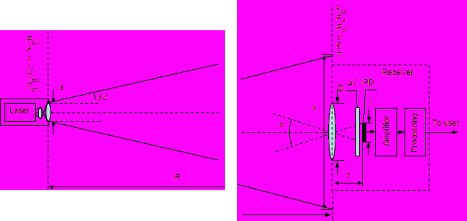
The model is written as a combination of Simulink blocks and Matlab code in a modular fashion. The basic methodology can be seen in Figures 1a and 1b, which depict the whole system from the laser source where the signal is generated, through to the receiver which represents the laser warning receiver and/or the laser missile seeker.

Laser sensor functioning mathematical model

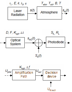
Knowing the general picture of the laser sensor, we need to introduce the mathematical formulae that are the basis for the model and analysis. Figure 2 shows the functioning mathematical model of the laser sensor.

Figure 1. Laser source and laser receiver/seeker.

Figure 2. Laser sensor functioning mathematical model.

Laser source gaussian pulse

Many optical systems, exhibit pulse outputs with a temporal variation that is closely approximated by a Gaussian distribution. Hence that variation in the optical output power (P₀(t)) with time may be described as [2]:

P_{0} (t) = \frac{1}{\sqrt{2 π}} e^{- (\frac{t^{2}}{2 σ^{2}})}

(1)

where σ and σ² are the standard deviation and the variance of the distribution respectively, and t represents current time. In our model, Figure 2, the output signal from the laser source s(t) is:

s (t) = P_{out} exp {- t^{2} / 2 σ^{2}}

;

σ \approx τ

(2)

where:

P_{out} = \frac{E}{τ}

(3)

E is the energy of the pulse, and τ is the pulse width.

This equation is the basis of the first subsystem in the sensor model and describes the radiation (emission) source parameters for example: power from mW to MW and pulse duration in nanoseconds.

Laser signal passed through the atmosphere

From Figure 2, the signal at the input to the sensor is:

s_{in} (t) = s (t) T_{A} (λ)

(4)

and T_A(λ) represents the atmospheric transmission for the laser path [3].

T_{A} (λ) = T_{A}^{abs} (λ) \cdot T_{A}^{sct} (λ)

(5)

Atmospheric transmission is an important factor to be considered and it consists of two components, absorption and scattering. In addition, the atmospheric attenuation is not uniform and is a function of wavelength. We consider the absorption first. The atmospheric absorption attenuation can be calculated using the following equation [3]:

T_{A}^{abs} (λ) = exp (- α_{abs} (λ) \cdot R)

(6)

where:

α_{abs} (λ) = α_{abs . H_{2} O} (λ) + α_{abs . {CO}_{2}} (λ) + α_{abs . O_{3}} (λ)

(7)

for λ =1.06 μm, which is one of the most important wavelength to cover in our study:

α_{H_{2} O} >> α_{{CO}_{2}}; α_{O_{3}}

(8)

The radiation absorption coefficient of water vapour in the atmosphere on a horizontal path is given by:

α_{abs . H_{2} O} (λ) = f (ω_{0}; E_{E}; T^{\circ}; H %)

(9)

where:

ω₀—the quantity of precipitable water (H₂O) (mm) over a distance of 1 km.

E_E—aqueous tension, Pa (7×10^-3… 1.2×10^-2 Pa);

T°—atmospheric temperature, K (300 … 330 K); and

H%—relative air humidity.

Secondly, the atmospheric scattering attenuation can be calculated and is given by:

T_{A}^{sct} (λ) = exp (- α_{sct} (λ) \cdot R)

(10)

For laser radiation scattering we need to consider the following three cases:

a) Clear atmosphere (R_m ≥ 10 km) [4]:

α_{sct} (λ) = \frac{3.91}{R_{m}} {(\frac{λ}{0.55})}^{- 0.585 \cdot \sqrt[3]{R_{m}}}

(km^-1) (11)

where R_m is the meteorological range (km); and λ is the wavelength of irradiation (μm).

b) Haze conditions: $α_{sct} (λ) = f (d, N)$ where d is the radius of particles, and N is the density of particles.

c) Fog conditions: $α_{sct} (λ) = f (d, N)$

The second subsystem of the model is designed to describe the influence of the atmosphere on the laser beam according to Equation (5). This subsystem is constructed from elementary blocks of Simulink and calculation of the atmospheric coefficients for absorption and scattering are done using LOWTRAN VII code.

Optical system

As seen in Figure 2, the signal at the entrance of the photodiode is given by:

s_{in 2} (t) = s_{in} (t) \frac{S_{PD}}{S_{beam}}

(12)

where:

S_{PD} = \frac{π \cdot D^{2}}{4}

(13)

is the area of sensing element of the photo detector.

S_{beam} = \frac{π \cdot {(a + θ \cdot R)}^{2}}{4}

(14)

S_beam—the sectional area of the laser beam at distance R from the laser source (without turbulent influence) where:

a—diameter of the transmitting objective; and

θ—divergence of the laser beam (typically between 2~5 mrad).

The third subsystem of the model describes the effect of the receiving optical system on the signal coming from the threat according to Equation (12).

Noise power

A very important issue for analysis is the noise. We have two sources of noise: external noise and internal noise. The external noise is due to factors such as the weather conditions, type of background, solar irradiance. The internal noise is due to electronic factors such as thermal noise and shot noise. These factors are discussed in more detail in Part II of this series of papers.

The noise input power to the photodetector is given by:

S_{n} (t) = P_{Σ} \cdot n

(15)

where n(t) is white Gaussian noise, and:

P_{Σ} = P_{b} + P_{r}

(16)

where the receiver channel noise power can be calculated as:

P_{r} = \frac{\sqrt{{\bar{i}}_{n}^{2}}}{S_{λ}}

(17)

(i_nis defined in more detail when we discuss threshold and decision making later in this paper) and the exterior irradiation power is given by:

P_{b} = [\sum_{i = 1}^{4} B_{i}] {ω Δ λ S}_{D} K_{opt}

(18)

where:

ω—the field of view of the receiver;

∆λ—the optical bandwidth of the system;

S_D—the input lens area;

K_opt—the transmission coefficient of the optical system (typically 0.4 to 0.6); and

B_i—spectral brightness and consists of four cases—direct solar, indirect solar, clouds, and dark sky (this is discussed in more detail later in this paper).

After the third subsystem there is an ‘adder’ which sums the useful signal from the laser source with the noise signals. The noise source is described by a Gaussian distribution. Furthermore, the blend of an optical signal and noise goes on as an input to the photodetector, which transforms the optical signal into an electrical signal.

Photodiode output

The photodetector is responsible of converting the received signal to a useful electrical signal which can be then transferred to the processing circuitry. The following equation is used to evaluate the behaviour of the photodiode:

U_{phd} (t) = S_{λ} [S_{in 2} (t) + S_{n} (t)] R_{L}

(19)

where:

$S_{λ}$ —the photodiode spectral sensitivity, and

$R_{L}$ —the load resistance.

Since we are looking to detect weak optical signals at long ranges we need to choose a photodiode with a high responsitivity. We are covering a wide optical bandwidth from 0.4 µm to 1.7 µm which will therefore require more than one photodiode.

The selection of a photodiode (APD or PIN) is defined by the requirements of the parameters of the receiving channel. If high sensitivity is required an APD is the best choice (due to its 50 to 200 times greater responsitivity). If a low noise level is required, a PIN photodiode would be a good choice. In this scenario it is necessary to use an APD as it allows for detection of low power laser sources at greater range.

The properties required from a photodiode (and that of the associated amplifier) are:

1. High responsivity (A/W).

2. Good linearity.

3. Wide bandwidth.

4. Low noise.

Amplification stage

The output voltage from the amplification stage may be described by:

U_{out} (t) = K \cdot U_{phd}

(20)

The amplification path is modelled on two cascade circuits. The typical pulse width for the optical signal in the model is 30 ns which makes the typical bandwidth requirement 33 MHz. Frequency filters for both amplifiers are built from standard blocks of Simulink libraries «Analog Filter Design ». In conjunction, they limit the region of amplification to between 0.9 MHz (low-frequency noise cut-off) to 33 MHz (corresponding to the signal pulse width). Butterworth filters have been utilised because of the required uniform shape of the amplitude-frequency characteristic (AFC), the simplicity in use of cut-off frequency definition and the filter order defines the slope of the AFC.

In practice, typical timing comparators, which are used as the decision device in a LWR, require an input signal of the order of 100 mV. As the noise equivalent power (NEP) of typical photodiodes are ~10 pA/Hz which yields a minimum perceived voltage of approximately 1.5 mV. Therefore the overall gain factor of amplification section should be of the order of 70…80 (100 mV / 1.5 mV).

The1st amplifier (prime amplifier) is represented in the model as an ideal amplifier with fixed amplification factor (equal to 4) which is connected in series with a highpass filter (Butterworth filter of second order with a cut-on frequency of 0.9 MHz) and a high-voltage limiter block to prevent saturation in the amplifier cascade.

The second amplifier is implemented in series with the first amplifier with a fixed amplification factor (equal to 20), a voltage limiter block, and a lowpass filter (Butterworth filter of second order with cutoff frequency of 33 Mhz).

Threshold voltage & decision making

The threshold voltage is given by:

U_{thresh} = P_{thr} \cdot S_{λ} \cdot R_{l} \cdot K \cdot q (D, F)

(21)

where q(D,F) is the signal-to-noise ratio, which provides required values of probability of correct detection (D) and a false alarm (F).

The receiver channel threshold power is calculated by the following equation:

P_{thr} = \frac{\sqrt{{\bar{i}}_{n}^{2}}}{S_{λ}}

(22)

where:

${\bar{i}}_{n}^{2}$ —the dispersion of the noise current, and

S_λ—the spectral sensitivity of photodetector, A/W.

The dispersion of the noise current consists of several current noises, the largest of which are the thermal and shot noises.

{\bar{i}}_{n}^{2} = {\bar{i}}_{therm . n}^{2} + {\bar{i}}_{shot . n}^{2} + {\bar{i}}_{tother . n}^{2}

(23)

{({\bar{i}}_{therm . n}^{2}; {\bar{i}}_{shot . n}^{2} >> {\bar{i}}_{tother . n}^{2})

where the thermal noise of the receiver is given by [5]:

{\bar{i}}_{therm . n}^{2} = \frac{4 \cdot k \cdot T \cdot Δ f}{R_{L}}

(24)

k—Boltzmann’s constant; and

T—the environmental temperature (typically 300–330 K).

and the receiver electronic bandwidth is given by:

Δ f \approx \frac{1}{τ}

(25)

As before, R_L is the load resistance of the photodetector (which is typically 10⁴–10⁵ Ω).

From the thermal noise equation we can see that it is possible to reduce this noise by increasing the value of load resistor. However, increasing the value of the load resistor to reduce the thermal noise reduces the receiver bandwidth. Optimization of the model parameters will lead to better performance.

The photodetector shot noise can be given by [5,6]:

{\bar{i}}_{shot . n}^{2} = 2 \cdot e \cdot Δ f \cdot ({\bar{I}}_{D} + S_{λ} \cdot {\bar{P}}_{A} + S_{λ} \cdot {\bar{P}}_{back})

(26)

where:

e—electron charge;

${\bar{I}}_{D}$ —average dark current ( ${\bar{I}}_{D}$ = 0.5...5 nA); and

${\bar{P}}_{A}$ —average power of optical signal, W.

The total contribution of the clutter/noise from all the background sources may be expressed as [3]:

{\bar{P}}_{back} = \int_{λ_{1}}^{λ_{2}} B (λ) \cdot ω \cdot S_{D} \cdot k_{opt} \cdot d λ

(27)

where:

B(λ) is the spectral brightness of the sky, W/cm²·µm·sr such that:

Day: B_D(λ) = 1.2·10^-3 W/cm²·µm·sr; and

Night: B_N(λ) = 10^-10 W/cm²·µm·sr.

From the scenario geometry (Figure 1b), the field of view of the receiver is given by:

ω = \frac{π \cdot ℓ^{2}}{4 \cdot f^{2}}

(28)

where:

$ℓ$ —size of sensitive area of photodetector (typically 0.2 to 1 mm);

f—objective focal length;

∆λ —optical bandwidth; and

k_opt—transmission coefficient of the optical system (typically 0.4 to 0.6).

and the area of the receiving objective is given by:

S_{D} = \frac{π \cdot D^{2}}{4}

(29)

After amplifying, the signal must be compared to a certain value (the threshold) to decide if there is detection or not.

Calculation of the threshold value is based on an estimation of the noise level of the whole system as shown in the equations above. If the signal amplitude exceeds the level of the calculated threshold, a square pulse will be generated at the oscilloscope indicating that the threat is detected.

Sources of solar background conditions can be seen in Figure 3. It is one of the more, if not the most, significant sources of noise the model should be capable of dealing with, particularly with respect to conditions expected in the UAE.

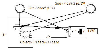
Four cases are considered, namely: direct solar illumination, diffuse reflection of typical surfaces (such as desert sand), diffuse reflection of cloud surfaces, and night sky radiation.

Three samples of UAE desert sand have been tested to generate their diffuse reflectivities over the wavelength range of interest and any of these values can be used as the background in the model.

The total contribution of the clutter/noise from all the background sources may be expressed as:

P_{b} = \sum_{i = 1}^{4} B \cdot ω \cdot Δ λ \cdot S_{Re ceiver} \cdot K_{optics}

(30)

and B_i, as defined earlier in Equation (19), is the spectral brightness, which is composed of four terms as follows:

\sum_{i = 1}^{4} B_{i} = μ \cdot I_{0} \cdot \frac{cos (ψ)}{π} + μ \cdot I_{0} \cdot \frac{cos (ψ)}{π} \cdot ρ + μ \cdot I_{0} \cdot k_{Clouds} + B_{N}

(31)

In this formula:

1. The first term is the direct solar illumination.

2. Second term is the diffuse surface reflection.

3. Third term is the diffuse cloud reflection.

4. Fourth term is the night sky radiation.

The parameters included in the equation are:

ρ—reflection coefficient from surface. A typical value of ρ = 0.02 to 0.3.
k_Clouds—reflection coefficient from clouds. A typical value of k_Clouds = 0.001 to 0.2.
B_N—spectral brightness of night sky (B_N = 10^-10 W/cm²·µm·sr)
µ—the coefficient describing the distribution of brightness depending on the solar angle in the sky and the observation angle. A typical value for µ is 0.172.
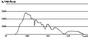
I₀(λ)—flux density of sunlight and can be seen in Figure 4 [3]. However, the model takes its values for I₀(λ) from the LOWTRAN computer code.

Conclusion

In this paper we have introduced the Laser Sensor Model as a theory and mathematical equations. Each part of the laser sensor has been explained and discussed in some detail to provide the base for building the model using MATLAB, Simulink, and the LOWTRAN VII computer code.

In Part II we show the detail of the graphics user interface (GUI) and demonstrate the model outputs.

In Part III we compare the model results to laboratory-based experiments and the results from some field trials, with real systems, in the UAE. This will demonstrate the validity of the model which will hence enable realistic predictions for optimisation of LWRs and countermeasure analysis to be carried out. This process is reported in the final Part IV of the series.

References

[1] D.H. Pollock, “Countermeasures Systems”, The Infrared & Electro-optical Systems Handbook, Vol. 7, SPIE Press, 1993.

[2] J.M. Senior, Optical Fiber Communications Principles and Practice, Prentice Hall, p. 544, 1985.

[3] R.G. Driggers, P. Cox, and T. Edwards, Introduction to Infrared and Electro-Optical Systems, Artech House, p. 407, 1999.

[4] D.P. Woodman, “Limitations in Using Atmospheric Models for Laser Transmission Estimates”, Applied Optics, Vol. 13, pp. 2193–2195, 1974.

[5] G.R. Osche, Optical Detection Theory for Laser Applications, John Wiley & Sons, Hoboken, New Jersey, 2002.

[6] M.A. Richardson, “Electro-Optical Systems Analysis—Part 1”, Journal of Battlefield Technology, Vol. 5, No. 2, pp. 24–26, July 2002.

Authors

Major Mubarak Al-Jaberi graduated with BSc in Electronic Engineering from George Washington University in 1998 and worked in the armament department of United Arab Emirates Army for several years. He is pursuing a doctoral programme on laser warning systems, laser-guided missiles and techniques at the Defence Academy of the United Kingdom.

Dr Mark Richardson is the head of Electro-optics group at the Defence Academy of the United Kingdom.

Dr John Coath and Dr Robin Jenkin are both lecturers at the Defence Academy of the United Kingdom.