
Volume 9, Number 1, March 2006
Gun Barrel Models For Use In Weapon Control System Investigations
- 1 Engineering Science Department, Defence College of Management and Technology UK , Cranfield University, Shrivenham, SN6 8LA, UK.
Abstract
In the design of Weapon Control Systems (WCS) for main battle tanks there is a requirement for low-order models of the elevating mass and barrel. In this work two models suitable for this requirement are put forward. The two models under consideration break the barrel down into rigid sections that are connected by frictionless pin-joints and linked by torsional springs and dampers. This model is referred to as a Lumped Parameter Flexible Beam Model (LPFBM) in this work. These models consider the barrel being broken down into two and three rigid sections. The lengths of the rigid sections and spring stiffnesses are selected to preserve the resonances (poles) and anti-resonances (zeros) of the system. This is achieved by using a novel scheme based on equations derived for the cantilever mode frequencies for the zeros and on optimising the lengths of the rigid sections for the poles. The responses from these two models, in the frequency and time domain, are compared to a finite-element barrel version, which is used as the base model and a non-optimised two-section LPFBM. Recommendations are then made on the appropriate model to use in the design of a WCS based on the required frequency range of the model and whether muzzle motion predictions are needed.
Nomenclature
| A | System matrix |
|---|---|
| B | Input matrix |
| C | Damping or output matrix |
| c | Damping coefficient |
| D | Transmission matrix |
| f | Force |
| I | Input or unit matrix |
| J | Performance index |
| K | Stiffness matrix |
| k | Stiffness |
| l | Length defined in Figure 1 |
| M | Mass matrix |
| m | Mass |
| Rp | Pinion radius |
| Td | Drive torque |
| u | Input vector |
| W | Weight |
| Xtp | Length defined in Figure 1 |
| x | State vector |
| x | Coordinate defined in Figure 1 |
| y | Trunnion vertical motion |
| β | Proportional damping coefficient |
| η | Length defined in Figure 1 |
| θ | Angular rotation |
| ω | Angular velocity or frequency |
| Superscript | |
| fe | Finite element |
| II, III | Two-section, three-section LPFBM model |
| o | Optimised |
| Subscript | |
| 1, 2, 3 | LPFBM section |
| 2, 3 | Two-section, three-section LPFBM model |
| 12, 23 | Between sections 1 and 2, 2 and 3 |
| b | Barrel or beam |
| c | Cantilever |
| d | Drive |
| m | Model, elevation |
| p | Platform |
Introduction
For Weapon Control System (WCS) investigations for Main Battle Tanks (MBTs) a model of the gun barrel/elevating mass is required that faithfully reproduces the motions of the system up to the highest frequency of interest, commonly 50–100 Hz. In this work two optimised barrel models are proposed for such studies and compared with both finite-element and non-optimised barrel models.
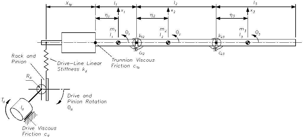
Three of the models consist of breaking the barrel down into two or three rigid sections that are pin-jointed together and linked by rotary springs and dampers. In this work these models are referred to as Lumped Parameter Flexible Beam Models (LPFBMs). A diagram for the elevation axis of an electrical drive MBT is shown in Figure 1, which has a three-section LPFBM. The modelling method proposed for the barrel can be applied to the traverse and elevation axes, the resulting order of the models, including the drive and turret inertias, being in the range from six to ten. With this relatively low order of model it is possible to run them in real time, as part of a prediction or estimator algorithm.
The modelling and control of flexible structures has received considerable attention [1–13], with the finite-element method having become the most common for gun dynamics investigations. The problem with finite-element models for control system studies is their relatively high order, which necessitates some form of model order reduction, though it does result in high-fidelity models [6–8].
For an insight into the dynamics of flexible structures it is possible to generate analytical models for simple structures [1,3,5,6]. These models show that the response consists of both resonances (poles) and anti-resonances (zeros). The poles are independent of where on the structure a measurement is made. While the zeros are dependent on the measurement position and can be thought of as resonances (poles) of a constrained sub-structure [9]. This can be explained as follows; consider a balanced elevating mass, which is pivoted at its trunnions and has no damping. The frequencies at which the motion of the breech is stationary (zero or anti-resonance) correspond to the cantilever frequencies of the elevating mass, this is a constrained sub-structure of the system. Also if measurements are made at the tip (or off the axis of rotation) of the flexible structure then the zero or zeros are in the right-hand side of the s-plane. In this case the response is non-minimum phase and is characterised by a step response that initially goes in the opposite direction.
To improve the fidelity of the LPFBMs in this work an optimisation process is proposed that attempts to preserve both the cantilever and as mounted frequencies of the elevating mass. A model that includes a finite-element barrel model is used as a base to which the others are compared. Both frequency and step responses for the elevation axis are presented for the drive, breech and muzzle motions and recommendations are made as to which model to use.
| Mode | Cantilever Hz (rad/s) | Pivoted at Trunnions Hz (rad/s) |
|---|---|---|
| 1 | 10.84 (68.11) | 0 (0) |
| 2 | 48.04 (301.84) | 19.74 (124.03) |
| 3 | 121.03 (760.45) | 52.12 (327.48) |
| 4 | 229.81 (1,443.94) | 122.68 (770.82) |
| 5 | 375.16 (2,357.20) | 230.67 (1,449.34) |
Models
In this section the modelling of the elevation axis is performed on a generic elevating mass/gun barrel, which has been taken from [10]. The data for the elevating mass is given in Appendix A, with some corrections from the original. A diagram of the elevation axis mechanics, with a three-section LPFBM is shown in Figure 1. In this model the drive-line flexibility has been collected together and placed between the elevating mass and the rack and pinion [5,6,8].
Finite element model
The finite element model is generated using the techniques given in [6–8] and consists of breaking the flexible barrel into ten Euler-Bernoulli beam elements. The model frequencies for both the elevating mass pivoted at the trunnions and with the cradle/breech held rigidly (cantilever) are shown in Table 1 for the first five mode frequencies. From this table it can be seen that the pivoted modes start at zero, representing a solid body rotation of the elevating mass about the trunnions. Also the nth cantilever frequencies get closer to the n+1th pivoted mode frequencies, for example the 9th cantilever frequency is 1341.6 Hz while that for the 10th pivoted is 1341.8 Hz, this is discussed in more detail in [1,5,6].
Lpfbm
In this part the LPFBMs are developed, the three-section version is done in detail, while the two-section model is just presented. This section finishes by considering the optimisation of both the LPFBMs.
Three section
A diagram of the three-section LPFBM is shown in Figure 1, if the drive-line is ignored. The cradle, breech and gun barrel (elevating mass) in this model are represented by three rigid sections, of length l1, l2 and l3, mass m1, m2 and m3, and moment of inertia about the centre of gravity I1, I2 and I3. The distance to the centres of gravity are η1, η2 and η3, the pin-joints linking the sections having torsional stiffnesses of k12, k23 and viscous friction c12, c23. The breech and muzzle motions are given by θ1 and θ3. This type of flexible beam model has been used to simulate and control flexible space-borne manipulators [11,12] and to investigate the design of WCSs [6,10,13].
The main assumptions built into the model are:
- All motions are small.
- The rigid sections are pin-jointed together by fictitious frictionless joints.
- All springs and dampers are linear.
- No longitudinal motions or forces are considered.
- Platform/mounting is stationary.
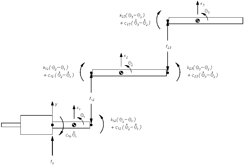
A free-body-diagram of the system is shown in Figure 2, where the force fy is the vertical force at the trunnions and y is the vertical motion of the trunnions, the vertical forces at the pin-joints are f12 and f23. The equation of motion for the three sections are:
Section 1:

Section 2:

Section 3:

Equations of constraint for the three sections are:

The equations of motion for the system can be written in matrix form, after eliminating the linear co-ordinates, as:

Where the mass, damping and stiffness matrices are given by:
and the vector of motions by:
The barrel damping for all the models, c12 and c23 in this case, is chosen to be proportional to the stiffness matrix using the following equation:
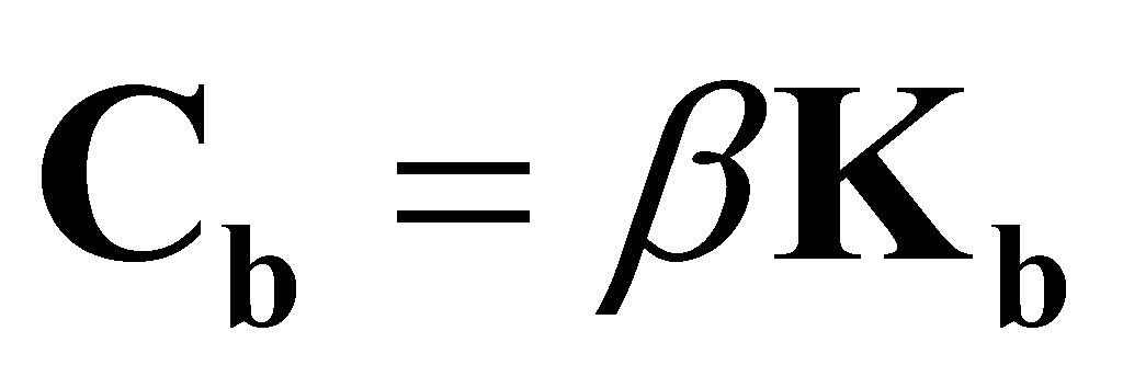
This is a common method of adding damping into structures [6–8].
Two section
Combining section two and three together in Figure 1, gives the two-section LPFBM, for which the equation of motion is:

where the mass, damping, stiffness matrices and vector of rotations are given by:
One method used for selecting the lengths of the rigid sections is given in [6,10,11], in which the muzzle displacement and rotation for the first cantilever mode is matched to the finite element model. The torsional spring rate is calculated to make the first cantilever mode frequencies of the LPFBM and finite-element models equal and is given by:

Optimising the lpfbm
For the LPFBM to have the same undamped zeros and poles, then its cantilever and pivoted (at the trunnions) frequencies must be the same as the real system, or in this case the finite element model. Equations for the cantilever mode frequencies can be derived for the LPFBM with both two and three sections, and from these the linking stiffnesses can be derived. For the two-section LPFBM this is given by Equation (8) above. The three section version is more complex and a symbolic manipulator has been used [14]. The cantilever modes are given by the eigenvalues of the matrix:
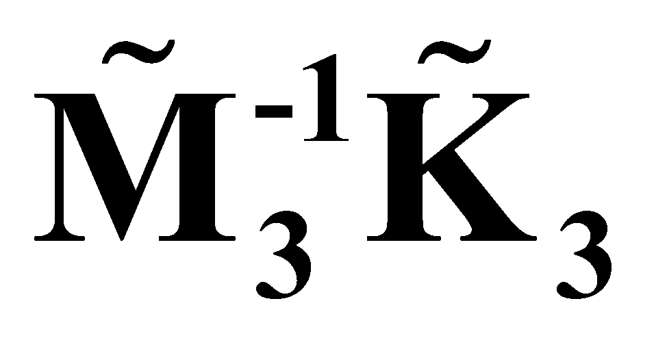
Where the ~ indicates that the matrices have had their first row and column removed, thus representing the cantilever case and:

where from Equation (5):
The two stiffnesses are determined to be:

where:
There are two possible solutions to these equations but only the first set (negative in the first and positive in the second) were found to give credible solutions, the reason for this being unknown.
The optimisation process [6] consisted of using the equations for the cantilever mode stiffnesses and altering the section lengths so that the mode frequencies for the elevating mass pivoted at the trunnions gave the frequencies of the finite element model. This was performed using the following cost function, which had to be minimised:
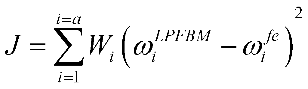
In this equation a = 2 for the two-section LPFBM and 3 for the three-section, Wi is a weight, which was taken as unity for all cases.
Care had to be taken to prevent the optimisation process homing in on local minima, by trying different starting lengths. In most cases the optimisation gave the same results, which are given in Table 2, for all the LPFBMs. Though this method has been used on a simple barrel model it is possible to use the finite-element description for real cases as is done in [6]. The resulting barrel stiffnesses are referred to as optimised and the superscript is augmented with an “o”. The optimisation process was performed using Matlab [14] with the built-in routines.
Elevation model
The elevation model is obtained by considering the complete system shown in Figure 1. The result is that the system matrices are augmented by the driveline and resulting matrices are [6]:
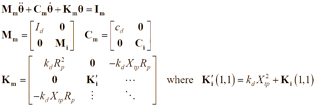
The input matrix is given by:
the vectors of rotations and input being:
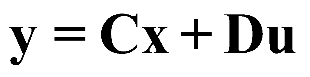
The models have been converted into state space form:
| LPFBM | |||
|---|---|---|---|
| Parameter | 2 Sect | 2 Sect Opt | 3 Sect Opt |
| m1 kg | 2165 | 2056 | 1947 |
| I1 kgm2 | 1090 | 663 | 431 |
| l1 m | 1.750 | 1.125 | 0.578 |
| η1 m | –0.465 | –0.568 | –0.647 |
| m2 kg | 335 | 443 | 306 |
| I2 kgm2 | 281 | 496 | 78 |
| l2 m | 3.250 | 3.875 | 1.761 |
| η2 m | 1.319 | 1.549 | 0.820 |
| m3 kg | – | – | 246 |
| I3 kgm2 | – | – | 135 |
| l3 m | – | – | 2.661 |
| η3 m | – | – | 1.116 |
| k12 MNm/rad | 4.00 | 7.23 | 16.00 |
| k23 MNm/rad | – | – | 6.03 |
where:
The input vector being the same as Equation (13).
Model Responses
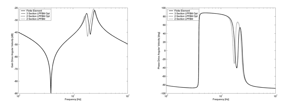
In this section the step and frequency responses are presented for the three models. The outputs considered are the drive angular velocity and the breech angle θ1 and muzzle angle θ2 or θ3, the input is the drive torque Td. The frequency responses have been determined between 1 and 100 Hz, though the muzzle motion is only presented from 10 to 100 Hz.
Frequency response
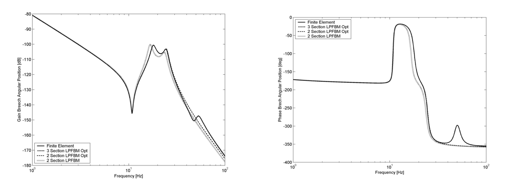
The drive angular velocity response, Figure 3, shows that there is little difference between the finite-element model and optimised LPFBM. The only discrepancy is with the non-optimised two-section LPFBM. In this case the zero at about 4 Hz is preserved but the two poles have some error associated with them. This error is removed with the optimisation as the section lengths have been adjusted to also achieve the same poles as the finite-element model.
For the breech angle, Figure 4, the non-optimised LPFBM shows the same error in predicting the poles, as would be expected but all models predict the first zero at 10 Hz. The optimised two-section LPFBM shows good correlation with the finite-element model up to 30 Hz. Above this some deviation exists and the zero/pole pair at about 50 Hz is not present. The three-section LPFBM follows the finite-element model up to the 100 Hz considered including the zero/pole pair at 50 Hz.
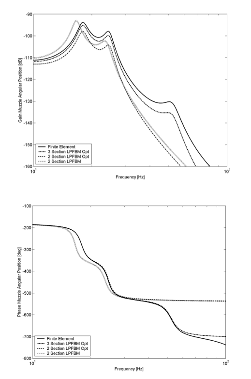
The muzzle angle response is more complicated, Figure 5 has been presented between 10 and 100 Hz to help highlight the differences. Ignoring the non-optimised two-section LPFBM, which has the same pole prediction errors. Both the optimised two- and three-section LPFBM show some deviation from the finite-element model in gain. The three-section model more closely follows the finite-element model including the pole at 50 Hz. For the phase, both the two-section models saturate at a phase lag of 540°. The three-section model follows the phase of the finite-element model to a phase lag of about 700°. The three-section LPFBM gives a reasonable representation of the finite-element response up to 30 Hz and to 60 Hz with a little more error.
Step response
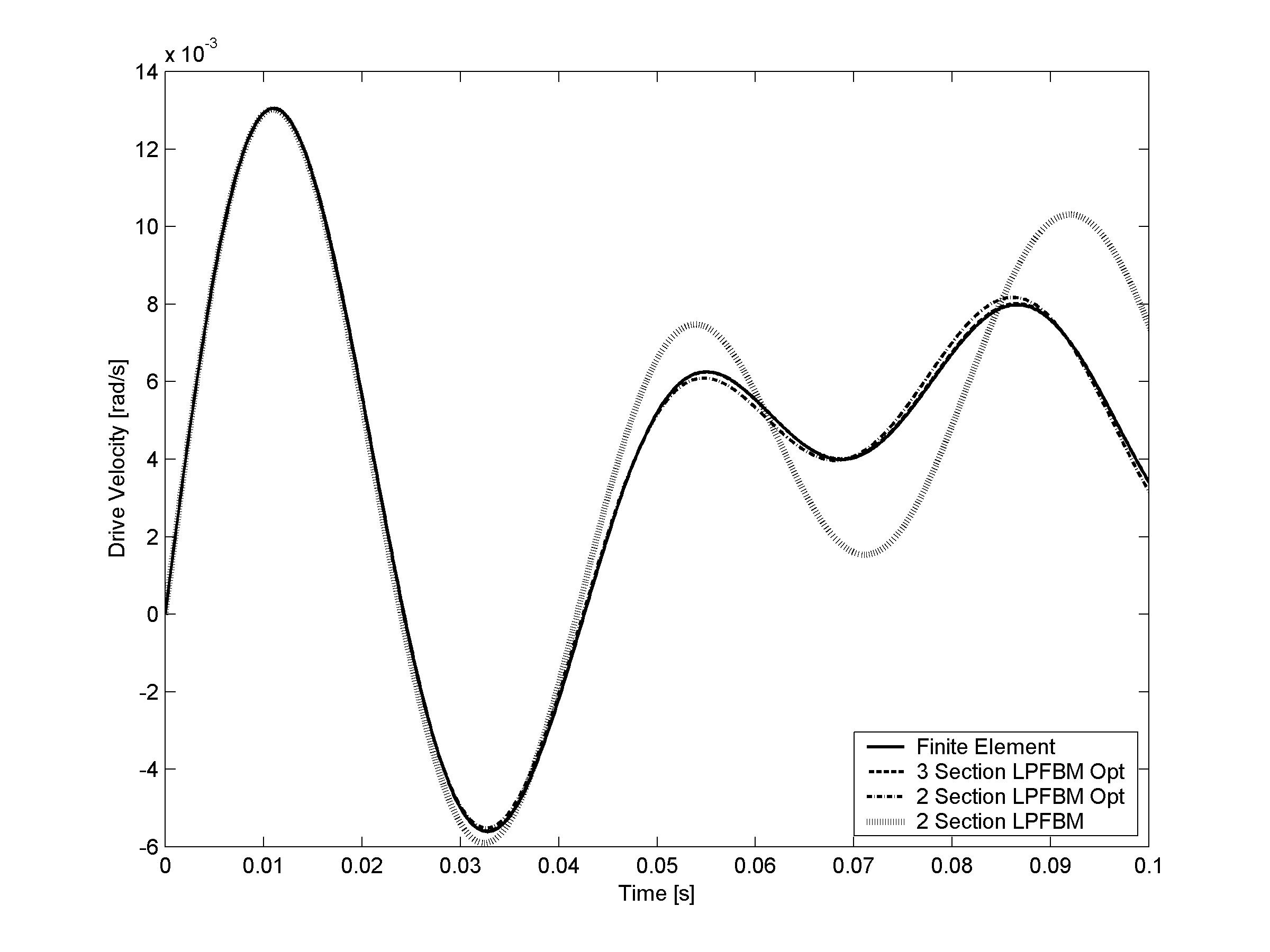
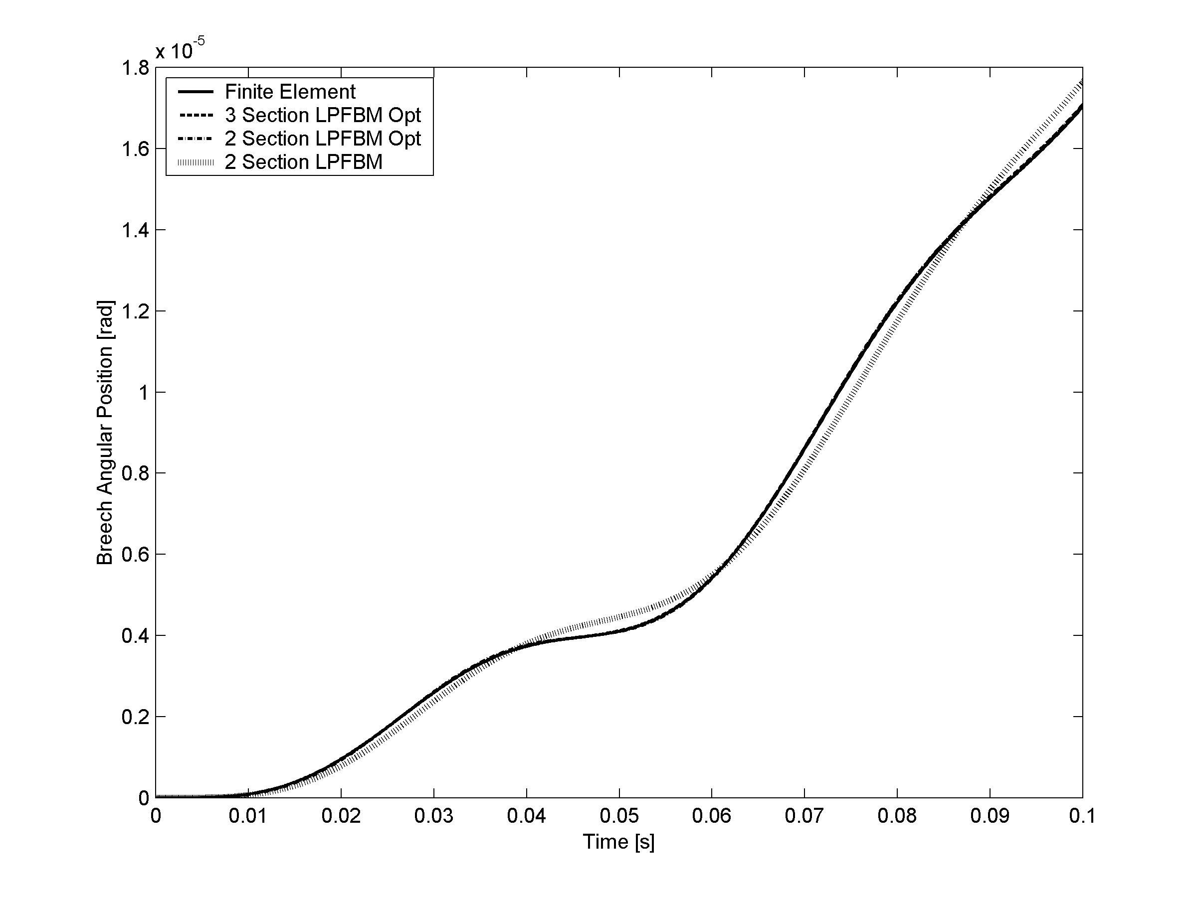
The drive angular velocity step response is shown in Figure 6. The only model that deviates from the finite-element model is the non-optimised two-section LPFBM, in which the motion has a larger amplitude and slightly lower frequency. The same can also be said of the breech angular response, Figure 7.
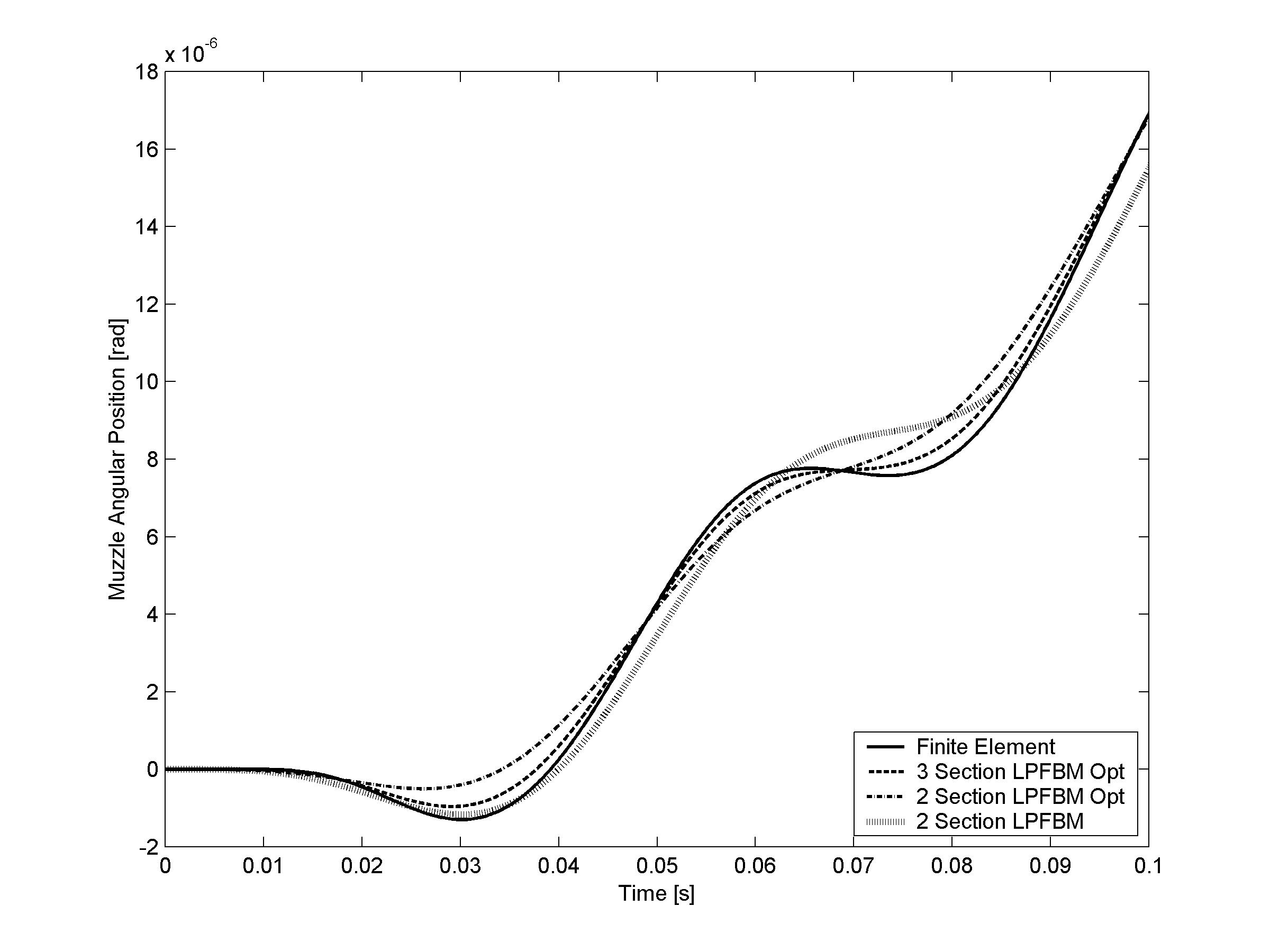
The most interesting response is that for the muzzle angle, Figure 8. In this figure the effect of the zero in the right half of the s-plane is clearly seen, with the response initially going in the opposite direction. This can be thought of a delay, thus making control of the muzzle a difficult problem [1,6]. The three-section LPFBM has the lowest over all error. Though, interestingly, the non-optimised two-section LPFBM predicts the initial motion best before having an increasing error.
Discussion
The non-optimised two-section LPFBM has been used successfully in the design of gun control systems [6,10] and prediction in a fire control system, though it has been shown here to give poor prediction of the system poles. The discussion here relates to the specific example of a 120 mm gun barrel, though an attempt is made to extend the results to a wider range of barrel sizes. This extension must be used with care and would need to be checked for the case being considered. The natural modes used for these predictions are taken from Table 1, for the pivoted at trunnions case.
For investigations up to about 30 Hz, which is 150 to 200% of the second mode, in both design and predictive purposes the optimised two-section model shows a good compromise between complexity and error. Its only significant error is in the muzzle motion.
The three-section model has good correlation with the finite-element model for both the drive and breech motions to over 100 Hz, or about 200% of the third mode. For muzzle motion the performance starts to deteriorate between 30 and 60 Hz, which is about 50 to 100% of the third mode. This type of model has been used in the design of a gun control system for both breech and muzzle motions in [6].
The frequencies given in this section are dependent on the actual frequencies of the gun barrel, which should not be too dissimilar to the generic model used here for main battle tanks. For other cases it would be prudent to verify the response of the resulting model.
conclusion
In this work four models of the elevation axis of a main battle tank have been presented with different representations for the gun barrel. Three of the models consider the barrel being broken down into rigid sections connected by pin-joints and linked by torsional stiffnesses and dampers. The final model used a finite element description of the flexible barrel.
A method for optimising the lengths of the rigid sections has been proposed, which has been shown to preserve the lower poles and zeros of the system.
It has been shown that optimising the barrel models significantly improves their accuracy in both the frequency and time domains.
Recommendations have been given for the use of the optimised models for a 120-mm MBT gun, thought care must be exercised if they are used for other gun calibres. These can be summarised as;
- For frequencies up to 30 Hz (or 150 to 200% of the second natural mode as mounted) and not including muzzle motion, the optimised two section model is the most appropriate.
- If muzzle motion is important or the frequency requirement is higher, then the optimised three section model would be best. The frequency range then being up to about 200% (100 Hz) of the third natural mode as mounted without muzzle motion or a maximum of 100% (60 Hz) with muzzle motion.
The non-optimised two-section model has been shown to have some errors in predicting the low-frequency poles but not the zeros.
| Model Parameter | Value |
|---|---|
| mr | 1818 kg |
| Ir | 308 kgm2 |
| ηr | 0.713 m |
| lb | 5.0 m |
| mb | 682 kg |
| Density ρ | 7,800 kg/m3 |
| Modulus of elasticity E | 209 GN/m2 |
| Id | 0.5 kgm2 |
| Rp | 0.04 m |
| kd | 6.0 MN/m |
| Xtp | 0.75 m |
| c1p | 1.5 kNms/rad |
| cd | 10 Nms/rad |
| Barrel stiffness proportional damping coefficient β | 0.0005 s |
References
[1] E. Schmitz, Experiments on the End-Point Position Control of a Very Flexible One-Link Manipulator, PhD. Thesis Department of Aeronautics and Astronautics Stanford University USA, April 1985.
[2] M. Spong, Control of Flexible-Jointed Robots: A Survey, Distributed Parameter Control Systems, New Trends and Applications, Lecture notes in pure and applied mathematics, Marcel Dekker Inc., 1991, ISBN 0-8247-8444-8.
[3] A. Fraser, and R. Daniel, Perturbation Techniques for Flexible Manipulators, Kluwer Academic Publishers, Dordrecht, The Netherlands, 1991, ISBN 0 79239 162 4.
[4] R. Sutton, G. Halikias, A. Plummer, and D. Wilson, “Modelling and H∞ Control of a Single-Link Flexible Manipulator”, Proceedings of the Institute of Mechanical Engineers, Vol. 213, Part (I), pp. 85–104, 1999.
[5] D. Purdy, “Theoretical Investigation into the Modelling of a Flexible Beam With Drive-Line Compliance”, Proceedings of the Institute of Mechanical Engineers, Vol. 216, Part (C), pp. 813–829, 2002.
[6] D. Purdy, An Investigation into the Modelling and Control of Flexible Bodies, PhD. Thesis, Cranfield University (RMCS), England, 1994.
[7] R. Cook, D. Malkus, and M. Plesha, Concepts and Applications of Finite Element Analysis, Third Edition, John Wiley & Sons, 1989, ISBN 88-27928.
[8] D. Dholiwar, “Development of a Hybrid Distributed-Lumped Parameter Open Loop Model of Elevation Axis for a Gun System”, Proceedings of the Seventh US Army Symposium on Gun Dynamics, Newport, Rhode Island, 11–13 May 1993.
[9] D. Miu, “Physical Interpretation of Transfer Function Zeros for Simple Control Systems With Mechanical Flexibilities”, Journal of Dynamic Systems, Measurement and Control, Vol. 113, 9/1991.
[10] D. Purdy, “Modelling And Simulation Of A Weapon Control System For a Main Battle Tank”, Proceedings Of The Eighth US Army Symposium On Gun Dynamics, 14–16 May 1996.
[11] P. Woerkom, On Fictitious Joints Modelling Of Manipulator Link Flexibility For The HERA Simulation Facility Pilot, National Aerospace Laboratory NLR The Netherlands, Report No. NLR TR 88086 U, 1988.
[12] M. Moch, and C. Kirk, Dynamics of Shuttle Based Flexible Antenna System, College of Aeronautics Report No. 9203, Cranfield University 1992.
[13] D. Purdy, “Main Battle Bank Stabilisation Ratio Enhancement Using Hull Rate Feedforward”, Journal of Battlefield Technology, Vol. 1, No. 2, July 1998.
[14] MATLAB/SIMULINK reference manuals, The MathWorks, Inc., 24 Prime Park Way, Natick, Mass.