
Volume 8, Number 3, November 2005
Combining Generic Structures and Systems Engineering to Manage Complexity in System Dynamics Modelling
Abstract
Expert system dynamicists are those who have developed the skills to perceive structure—that is, they have ability to recognise that dynamics appearing to be very different on the surface are actually caused by fundamentally similar mechanisms. They then use these skills very effectively to build models of complex problems. Desire to exploit knowledge of fundamental structures in system dynamics models has led to the formulation of molecules of system dynamics structure. But there is more we can do to facilitate learning about, and recognition of, structure as well as improve system dynamics modelling methodology. This paper argues that aspects of systems engineering practice can be integrated with system dynamics to produce a methodology which exploits knowledge of structures, utilises top-down model formulation and bottom-up construction of models, thereby enabling management of the complexity encountered during model building. The proffered methodology enables all modellers, even the least experienced, to quickly and reliably build robust models of complex problems. How this is achieved is explained and demonstrated.
Generic structures in system dynamics modelling
In ‘Industrial Dynamics’, Jay W. Forrester (1961: 2) recognised the importance of guiding system dynamics students to studying principles of structure and causes underlying dynamic behaviour:
The rapid strides of professional progress [in system dynamics modelling] come when the structure and principles that integrate [synthesise (in systems engineering terms)] individual experiences can be identified and taught explicitly rather than by indirection and diffusion. The student can inherit an intellectual legacy from the past and build his own experience upward from that level rather than having to start over again at the point where his predecessors began.
Paich (1985: 126-132) stresses an insight by Richmond that there could be considerable utility in isolating and defining ‘atoms of structure’, those ‘primitive feedback loops, which generate behaviour of basic processes’, which experienced system dynamicists recognise as important.
Since those formative times in the development of the system dynamics discipline, there have been a number of dedicated researchers and practitioners working to progressively identify and define these fundamental building blocks of structure. These building blocks have been variously referred to as ‘atoms’ (Richmond, 1977), ‘molecules of system dynamics structure’ (Hines, et al., 1996; 1997; 2000), ‘common modules’ (Coyle, 1996), ‘organelles’ (Malcszynski, 2005), and ‘modules’ (McLucas, 2005).
The term ‘molecule’ is used in the remainder of this paper to describe those building blocks of system dynamics structure defined by Hines et al. (1996; 1997; 2000) and McLucas (2005). The term module, which includes molecule, is used to describe the fundamental building blocks used during the process of building system dynamics models. Figure 1 illustrates how a molecule is defined in terms of a module boundary and inflows and outflows (McLucas, 2005).
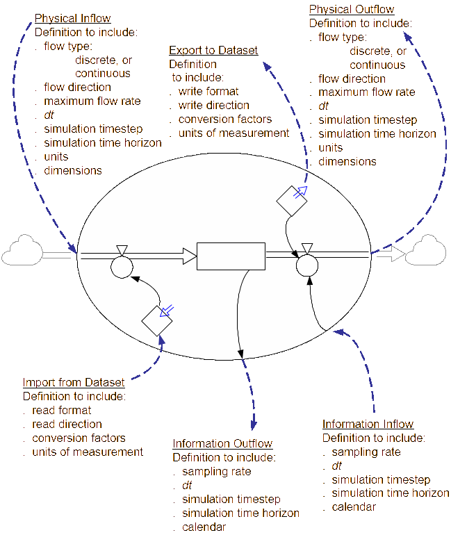
Whilst the import and export to datasets are important for the overall operation of the model, and this has to be verified at some stage, the interfaces (for the purposes of integrating with other modules, sectors or models) are:
- physical inflows,
- physical outflows,
- information inflows, and
- information outflows.
Many researchers and practitioners have had thoughts on generic structures along the lines of Graham (1977), Forrester (1968), Goodman (1989), Paich (1985) and Hines, et al. (2000). Significant contribution has been made by Coyle (1996) who makes repeated reference to, and provides examples of, ‘common modules’ which he has defined and described both as sets of influence diagrams and corresponding functional blocks of code in COSMIC® software. It is emphasised at this point that these functional blocks are not the algebraic definitions commonly encountered in system dynamics software, such as STEP, PULSE, or Delay.
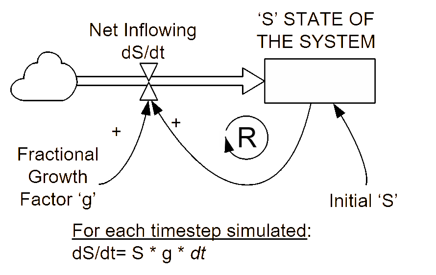
Perhaps the most familiar molecule of system dynamics structure is that defined by Sterman (2000: 266). This is the first-order linear positive feedback system, as depicted in Figure 2.
Depending on the exact definition of molecule used, it might be possible to define more than 50 functional building blocks (Hines, et al., 2000, define some 46 molecules).
Managing complexity with systems engineering
Traditional engineering design methods are based on a bottom-up approach in which known components are assembled into subsystems from which the system is constructed. The system is then tested for the desired properties and the design is modified in an iterative manner until the system meets the desired criteria. This approach is valid and extremely useful for relatively straightforward problems that are well defined. Unfortunately, complex problems cannot be solved with the bottom-up approach.
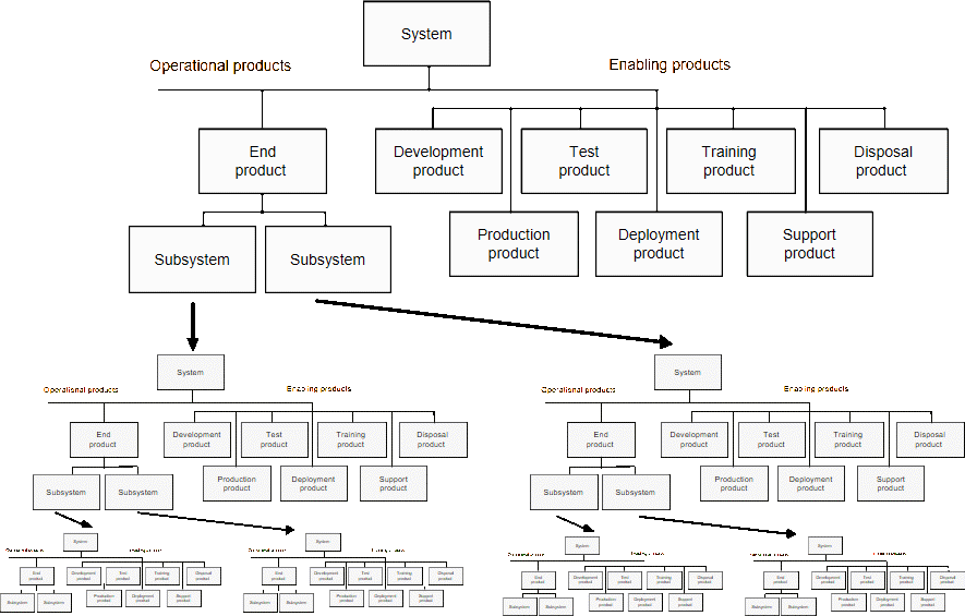
Systems engineering begins by addressing the complex system as a whole, which facilitates the initial allocation of requirements as well as the subsequent analysis of the system and its interfaces. Once system-level requirements are understood, the system is then broken down into subsystems and the subsystems further broken down into components until a complete understanding is achieved of the system from top to bottom. This top-down approach is a very important element of managing the development of complex systems. By viewing the system as a whole initially and then progressively breaking the system into smaller elements, the interaction between the components can be understood more thoroughly, which assists in identifying and designing the necessary interfaces between components (internal interfaces) and between this and other systems (external interfaces). For example, Figure 3 illustrates the ANSI/EIA-632 (1999) approach to top-down development.
It must be recognized, however, that while design is conducted top-down the system is implemented using a bottom-up approach. That is, one major aim of system engineering can be considered to be to provide a rigorous, reproducible process by which the complex system can be broken into a series of simple components that can then be designed and developed using the traditional engineering bottom-up approach. Importantly, the other major aim of systems engineering is to provide a process by which the components and subsystems can be integrated to achieve the desired system properties.
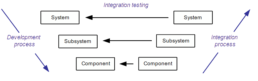
Integration (synthesis) aims to combine lower-level components into progressively higher-level subsystems until the system is complete. While the design process has been conducted top-down, the integration process is conducted bottom-up using well-proven techniques. At each stage of the integration, some form of integration testing is conducted to verify the successful integration against the appropriate level of documentation. Eventually, when systems integration is complete, testing can be conducted at the system level against the original requirements. Test and evaluation plays a role in all phases of the systems engineering effort. The integration effort is summarized in Figure 4. Note that the terms system, subsystem and component are relative. Each system comprises subsystems that consist of components. Each subsystem, however, can be considered to be a system in its own right, which has subsystems and components and so on.
Managing complexity in modelling
The use of modules therefore goes some way towards reducing the complexity of modelling. There is, however, much more to gain through an application of the top-down approach of systems engineering to the development of models. Before considering an example of such an application, this section addresses complexity and introduces a useful complexity measure.
There is considerable evidence that human cognitive capability is limited when dealing with dynamic complexity (Diehl and Sterman, 1995; Dörner, 1980; Forrester, 1971; Kleinmuntz, 1985; 1993; Mosekilde and Larson, 1988; Mosekilde, et, al., 1990; Paich and Sterman, 1993; Sterman, 1989a; 1989b; 1989c; 1994; 2000; 2002 and Sweeney and Sterman, 2000).
Before considering this further, let us introduce a metric for characterising the complexity of each molecule and any model of interest. Kline (1995) defines a complexity index, C:
V + P + L < C < V . P . L (1)
where:
V = number of state Variables which describe the system;
P = number of independent (non-zero valued) Parameters describing the system; and
L = number of feedback Loops describing the system.
For the molecule in Figure 2, C > 1 + 2 + 1 (= 4) ≈ 5.
Human cognitive capacity is limited to the analysis of problems where the complexity index, C, is not greater than 5. This limit has been suggested Sterman (2000: 39) and corresponds to Miller’s 7-bit rule (Miller, 1956), and is further argued by McLucas (2001; 2003). This practical limit has important implications for the way we set out to build and test models.
Let’s then look at the complexity of some selected system dynamics models, using the complexity index, C, as a means of comparison.
For molecules defined by Hines, et al. (1996, 1997, 2000), Table 1 lists the associated complexity indices, C. When modules (including molecules) are integrated (assembled) with other modules, the increase in complexity encountered derives directly from the interfaces between the modules.
This table categorises each of the molecules defined by Hines, et al. according to their complexity as measured by the Complexity Index, C. Some 26 of the molecules are characterised by C of 5 or less, suggesting that their structures and resultant dynamic behaviours are within our cognitive capacity (McLucas and Ryan, 2005). That is, they have complexity no greater than a first-order, linear positive feedback system whose dynamic behaviour (Sterman, 2000: 29) tests our cognitive capacity to the limit. The remainder of these molecules range in complexity from 6 to 480 and, therefore, have dynamic behaviour beyond our intuition.
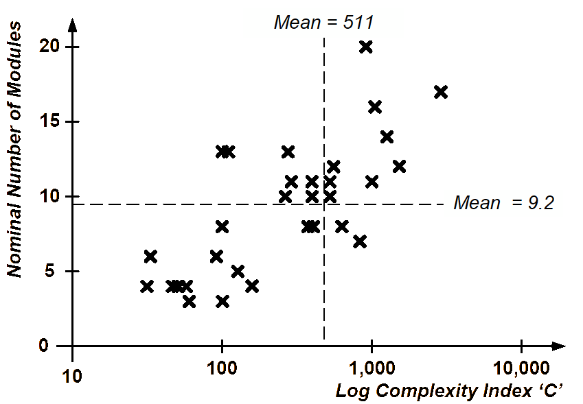
As another means of comparison, the authors analysed 30 models that have been described in detail in various peer-reviewed papers in the System Dynamics Review, published during the period 1985 to circa 1995 when publication of full code listings ceased. As illustrated in Figure 5, these selected exemplars of system dynamics modelling contain between four and 20 modules with a mean of around nine. The models analysed are characterised by C between 30 and 3000 with a mean of 511.
| Complexity Index, C | Count of Molecules | Molecule Names |
|---|---|---|
| 2 | 3 | Level, Residence Time, Producing. |
| 3 | 8 | Goal Gap, Decay, Resource Split, Ceiling, Dimensionless Input to Function, Floor, Market Share, Overtime. |
| 4 | 7 | Smooth, Material Delay, Conversion, Soft IF-THEN, Anchoring and Adjustment, Productivity, Estimated Completion Date. |
| 5 | 8 | Level Protected by Level, Normal Times Effects, Product Attractiveness, Desired Workforce, Workforce, Scheduled Completion Date, Anchor Pricing. |
| 6 | 5 | Cascaded Level, Co-Flow, Hines Co-Flow, Level Protected by Flow, Fatigue. |
| 7 | 3 | Present Value, Trend, Extrapolation. |
| 8 | 1 | Smooth Pricing. |
| 10 | 2 | Protected Anchoring and Adjustment, Protected Anchor Pricing. |
| 12 | 1 | Purchasing. |
| 14 | 1 | Inventory Ordering. |
| 16 | 1 | Inventory Backlog and Shipping Protected by Level |
| 24 | 1 | Inventory Backlog and Shipping Protected by Flow. |
| 32 | 1 | Diffusion. |
| 42 | 1 | Work Accomplishment Structure. |
| 54 | 1 | Ageing Chain. |
| 60 | 1 | Capacity Ordering. |
| 108 | 1 | Ageing Chain with PDY. |
| 480 | 1 | Cascaded Co-Flow. |
Typically problems analysed in this way have complexity in the order of 100 times greater than those we might reliably analyse without the benefit of system dynamics modelling. While the main models have significantly greater complexity than we can manage easily, further analysis of the models shows that they contain an average of nine modules each having complexity approximating the limit of our cognitive capability in handling complexity, that is, C is not greater than 5. It is obvious that experienced modellers have been able to model complex situations (that are beyond their cognitive capabilities) by integrating a manageable number of modules, each of which has manageable complexity.
Breaking a problem down to represent it as sets of modules is conceptually simple. Indeed, early users of applications such as DYNAMO® (which evolved from Fortran) were forced to have the discipline to build models using blocks of code. More recently, users of modelling applications with object-oriented graphical user interfaces with objects such as stocks (levels or accumulators), auxiliaries (converters) and flow-controlling valves, find it easy to construct modules (and models for that matter) from these components of system dynamics modelling.
Deciding how to analyse a problem situation and then define the requirements for the model, sectors and modules is not straightforward, however, particularly when a number of people are involved. Additionally, re-combining (assembling or integrating) modules / sectors / co-models is a significant challenge because of the potentially rapid introduction of complexity this brings. Systems engineering provides a suitable response to this challenge by providing methods for a top-down definition of the model and then a framework for the design of verification tests and the progressive application of these tests.
Consider the basic module shown in Figure 6. The problem being modelled, which has been defined in an earlier stage through a top-down analysis, involves a population whose growth is constrained by the ability of the environment to support it. As POPULATION increases, noting that a portion of the population is fertile and of an age where they might bear offspring—described by the Birthing Fraction ‘b’, we can develop a first-order positive linear feedback variant.
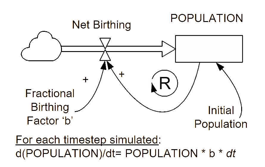
We can design and implement tests to assure that this evolving model behaves as it should. Here the model evolves through a series of structured processes with the aim of producing functionality identified as a consequence of a systems engineering top-down approach. It is always critically important (Forrester, 1961: 115-129) that the model explains the real world behaviour through the structure and equations, which reflect the real causal relationships in the real-world system.
The results of such testing can be confirmed in a number of ways including by comparing results obtained with the definition of the molecule and knowledge that without exogenous influence, exponential growth will be produced. Indeed, the purpose of system dynamics modelling software is to enable us to both build models and test them (verifying behaviour) for a range of parametric values.
The next stage of model development would involve analysis of the relationship between size of the population and carrying capacity. Again the complexity we are dealing with here is similar, although we are introducing a non-linear relationship. When non-linear relationships are introduced, we need to be more careful in the design of the test to verify that the model actually reflects the nature of the non-linearity. Of necessity, such tests must be more comprehensive, involving both logical and extreme-value testing. The feedback model under development would be as shown in Figure 7 and the non-linear relationship would be as shown with Population Divided by Carrying Capacity as the x-axis and Birth Rate Multiplier on the y-axis.
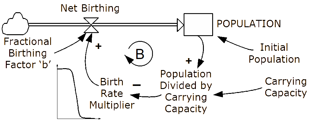
For the model under construction, Figure 7, C >1+3+1(=5)—that is, C ≈ 6.
Imagine, then, a more-complete consideration of our population model where we take into account the net dying rate as well as net birthing rate. The suggested form of the resultant model is depicted in Figure 8, with the additional non-linear death rate relationship. This example corresponds to that described by Sterman (2000: 285-288).
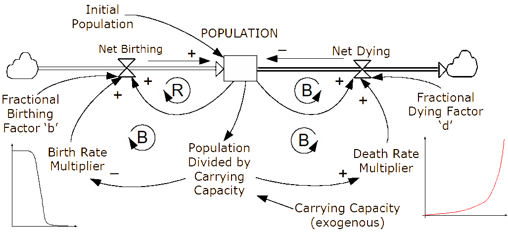
By our complexity measure, this model has a complexity index of C = 16 (that is 4×1×4), which is beyond the intuition of an individual and certainly stressing our ability as a group of humans to discuss the model and the relationships of its components. It is important to note that this model cannot be constructed bottom-up unless it is firstly conceptualised through a top-down approach (even if such a top-down understanding is only intuitively applied by the modeller). In turn, this can only be developed through a sufficiently detailed understanding of feedback dynamics and some considerable familiarity with the problem space and models of a similar (growth and decay) nature. Consequently, while the development of such a model is clearly possible for experienced practitioners, it is reasonable to expect that such a model can only be developed by someone who has experience in developing such a model (or at least something similar) before—this does not help us when employing less-experienced modellers or when facing problems we have not yet encountered. Despite the desirability (Sterman, 2000: 81) to use expert system dynamicists in model building, this is not always possible and our modelling practices should enable relatively inexperienced system dynamicists to build viable models.
Application of systems engineering to system dynamics modelling
Through a top-down approach, systems engineering provides the framework within which to consider the problem at a level of aggregation that keeps the model within a degree of complexity that does not exceed out cognitive capability (McLucas and Ryan, 2005). For example, Figure 9 illustrates a top-level view of a population model taking into account birthing and dying rates in the context of an environmental carrying capacity. Note that, in addition to the environmental effects on birthing and dying rates (Factor 1 in both modules), the designers could consider future expansion by allowing for other rate-effecting factors to be included (Factors 2…n in both modules).
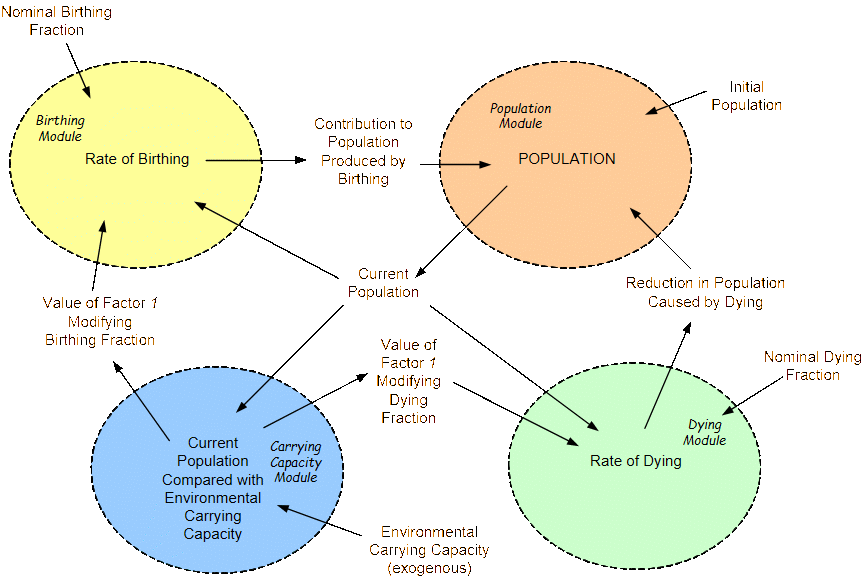
The major difference between Figure 8 and Figure 9 is that the complexity of the view has been reduced from C = 16 to C = 11, where the latter is determined by establishing the complexity encountered in consideration of any particular module. That is the Birthing, Population, Carrying Capacity and Dying modules have Complexity Indices of 3, 4, 2 and 2 respectively. This comes about by initially treating each module as a ‘black box’ with the result that the complexity arises from the interfaces with other models. Note that whilst feedback loops might exist when we consider the internal structure of the model, at this level of abstraction the problem becomes highly simplified as a result of that complexity being stripped away. It is also intuitively obvious that the population module will contain the key (state) variable POPULATION. This has that result that the modular view of the problem is within the cognitive capability of all participants in the initial problem-definition stage of the model design.
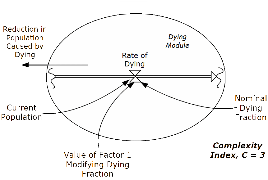
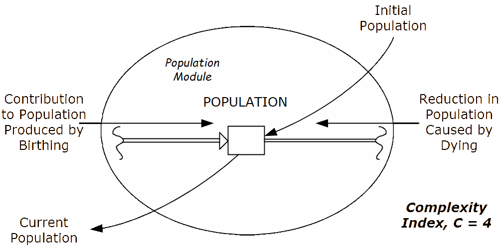
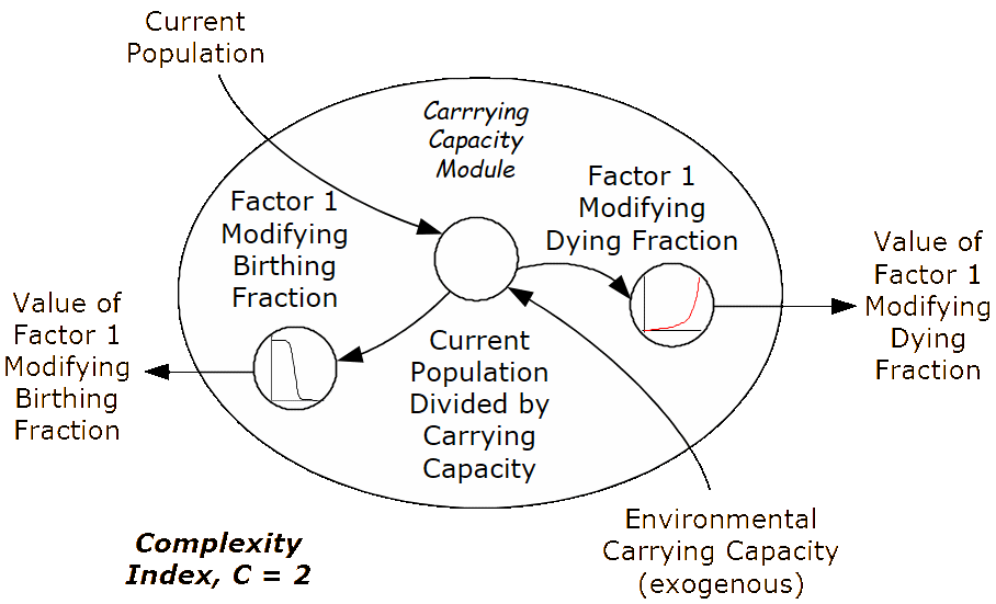
The process can now continue as each module of the model is now defined in terms of the required internal functionality as well as the necessary interfaces. For example, Figure 10 shows the further definition of the modelling elements of the four modules identified in Figure 9.
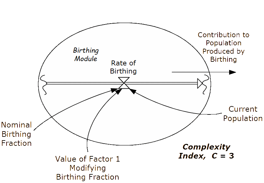
The four modules of the model each have complexity characterised by C<5. More importantly, the top-down approach would now allow us to allocate each of the modules to separate modellers to develop in isolation since we can provide them with a formal description of the internal functionality of each module and a statement of the necessary interfaces.
Having developed the modules, either by a single developer or a number, each module can be individually tested to ensure that it possess the required functionality. Then integration tests can confirm that each module is able to be integrated (as appropriate) with each of the other modules to which it must connect. Finally, the system can be constructed by integrating all four modules, and validation tests can confirm that the model performs as intended.
In general then, the top-down approach should be used to define the functional requirements of the model, including the system-level interfaces. The functionality is then allocated to sectors and the interfaces between sectors is defined. Finally, functionality within each sector is allocated to modules and interfaces between modules are defined. Each module is then given (along with the formal specification of the functionality of the module and its interfaces) to a nominated modeller who develops the module (possibly by utilising generic molecules) and then tests it to ensure that the module possesses the required functionality and interfaces (input and output flows) that are required. Modules are then integrated into sectors, which are then tested. Sectors are then integrated to create the model which is then tested for desired performance.
There are many other advantages to a top-down approach to design. Note for example in Figure 10 that the Birth Module and Death Module are almost identical—it would make sense to give these modules to the same modeller who can make the simple changes to the generic module to change it from the growth to the decay variant.
The stages of construction; Complexity Index, C, for each stage; and incremental increase in Complexity Index since preceding stage are depicted in Annex A. Annex A demonstrates how once the model to be built is broken down to functional modules, these are integrated (that is, assembled together with modules from earlier stages) to produce the final model. Before any stage can be completed, the module constructed must be tested (that is, functionality is verified against formally stated requirements). From one stage to the next, the incremental increases in C are kept small, preferably no greater than C=5, corresponding to our cognitive capacity and reliability when dealing with complexity.
Conclusions
The notion of structure underlying dynamic behaviour has been long recognised. Molecules of structure are now relatively fully described, though some further development is likely. The significance of modules (including molecules) in the development of system dynamics models is only fully recognised when a top-down design to building models is implemented. This top-down approach is drawn form systems engineering practice and has the added advantage that its judicious application assures we can build models using stepwise processes whereby we do not add complexity at any stage with the results that our cognitive capability to deal with complexity is not exceeded.
References
ANSI/EIA-632-1998, 1999, ‘Processes for Engineering a System’, Electronic Industries Association (EIA), Washington, D.C.
Coyle, R.G., 1996, ‘System Dynamics Modelling: A Practical Approach’, Chapman and Hall, London.
Diehl, E. and Sterman, J.D., 1995, ‘Effects of feedback complexity on dynamic decision making’, In: Organisational Behaviour and Human Decision Processes, Vol. 62, No. 2.
Dörner, D., 1980, ‘On the difficulties people have in dealing with complexity’, in: Simulation and Games. 11: 87-106.
Forrester, J.W., 1961, ‘Industrial Dynamics’, Productivity Press, Portland, Oregon.
Forrester, J.W., 1968, ‘Principles of Systems’, Productivity Press, Cambridge, Massachusetts.
Forrester, J.W., 1971, ‘Counter intuitive behaviour of social systems’, in: Technology Review No. 73, January: 52-68.
Goodman, M.R., 1989, ‘Study Notes in System Dynamics’, Productivity Press, Portland, Oregon.
Graham, A., 1977, ‘Principles on the Relationship Between Structure and Behaviour of Feedback Systems’, Ph.D. Dissertation, Department of Electrical Engineering and Computer Science, MIT, Cambridge, MA.
Hines, J., et al., (1996; 1997); 2000, ‘Molecules of Structure: Building Blocks for System Dynamics Models’, Version 1.4, LeapTec and Ventana Systems, Inc.
Kleinmuntz, D.N., 1985, ‘Cognitive heuristics and feedback in dynamics decision environment’, in: Management Science, Vol. 31, No. 6: 680-702.
Kleinmuntz, D.N., 1993, ‘Information processing and misperceptions of the implications of feedback on dynamic decision making’, in: System Dynamics Review, Vol. 9, No. 3 (Fall 1993): 223-237.
Kline, S.J., 1995, ‘Conceptual Foundations for Multidisciplinary Thinking’, Stanford University Press, Stanford, California.
Malcszynski, L. 2005, ‘Organelles of system dynamics structure’ in: Discussions on Powersimtools Group website. powersimtools@yahoogroups.com, February, 2005.
McLucas, A.C., 2003, ‘Decision Making: Risk Management, Systems Thinking and Situation Awareness’, Argos Press, Canberra, Australia.
McLucas, A.C., 2005, ‘System Dynamics Applications: A Modular Approach to Modelling Complex World Behaviour’, Argos Press, Canberra, Australia.
McLucas, A.C. and Ryan, M.J., 2005, ‘Meeting Critical Real-World Challenges in Modelling Complexity: What System Dynamics Modelling Might Learn from Systems Engineering’ in: Proceedings of International System Dynamics Conference, System Dynamics Society, Boston, MA.
Miller, G.A., 1956, ‘The magical number seven, plus or minus two: Some limits on our capacity for processing information’, Psychological Review, Vol. 63, No. 2: 81-97.
Mosekilde, E. and Larsen, E.R., 1988, ‘Deterministic chaos in the beer production-distribution model’, in: System Dynamics Review, Vol. 4, Nos. 1-2: 131-147.
Mosekilde, E, Larsen, E.R. and Sterman, J., 1990, ‘Coping With Complexity: Deterministic Chaos in Human Decision Making Behaviour’, in: J. Casti and A. Karlqvist (eds.), Beyond Belief: Randomness, Prediction and Exploration in Science. CRC Press, Boston, 1990.
Paich, M., 1985, ‘Generic structures’ in: System Dynamics Review, Vol. 1, No. 1: 126-132.
Paich, M. and Sterman, J.D., 1993, ‘Boom, bust, and failures to learn in experimental markets’, in Management Science, Vol. 39, No.12: 1439-1458.
Richmond, B, 1977, ‘Atoms: fundamental building blocks of sructure’, Personal communication with Mark Paich, circa 1977.
Sterman, J.D., 1989a, ‘Misconceptions of feedback in dynamic decision making’, in Organisational and Human Decision Processes, No. 43: 301-335.
Sterman, J.D., 1989b, ‘Modeling managerial behavior: Misperceptions of feedback in a dynamic decision making Experiment’, in: Management Science, Vol. 35, No. 3: 321-339.
Sterman, J.D., 1989c, ‘Misperceptions of feedback in dynamic decision making’, in: Milling, P.M. and Zahn E.O.K. (eds), International System Dynamics Conference: Computer-Based Management of Complex Systems. International System Dynamics Society, Stuttgart: 21-31.
Sterman, J.D., 1994, ‘Learning in and about complex systems’, in: System Dynamics Review, Vol. 10, No. 2-3, (Summer-Fall): 291-330.
Sterman, J.D., 2000, ‘Business Dynamics: Systems Thinking and Modelling for a Complex World’, Irwin McGraw-Hill.
Sterman, J.D., 2002, ‘All models are wrong: reflections on becoming a systems scientist’, in: System Dynamics Review, Vol. 18, No. 4, (Winter): 501-531.
Sweeney, L.B. and Sterman, J.D., 2000, ‘Bathtub dynamics: initial results of a systems thinking inventory’, in: System Dynamics Review, Vol. 16, No. 4, (Winter) 2000.