Mathematical Modelling of a Hydro-gas Suspension Unit for Tracked Military Vehicles

Nomenclature

Introduction

The design of suspension systems for military vehicles has always been difficult because of the conflicting requirements [1]. The main challenges are space constraints on the suspension, requirement for large wheel travel, and providing a rising rate spring. One of the suspension designs that permits a large amount of wheel travel and a rising rate is the hydro-gas system seen on the current (Challenger 2) and previous British main battle tanks [2].

One major advantage of the hydro-gas suspension system is the ease with which its spring and damping characteristics can be varied dynamically [2]. This capability has paved the way for developments towards active and semi-active control of the suspension to provide appropriate suspension parameters for different kinds of terrain.

Active and semi-active vehicle dynamics have become a subject of major interest during recent years, and simple damping control systems are incorporated in many modern passenger cars [3]. Rapid progress in the analysis, design and technology of the control systems leads to the need for an accurate description of the dynamics of all the components involved, such as, for instance, the tyre or shock absorber. It is only a matter of time before the technology will also be used for off-road military applications.

This work presents a method of simulating a hydro-gas unit, which incorporates the compressibility of the hydraulic fluid and the damper valve flow characteristics. This model is then incorporated into a mathematical model of a six-wheel station tracked vehicle. The ride performance of the vehicle for known inputs is investigated and a method is proposed for selecting the orifice diameter for the damper valve.

Hydro-gas suspension unit

Figure 1 shows the cross section of the Hydro-gas Suspension Unit (HSU), used on a British main battle tank, mounted on trailing arms. The system consists of a cylinder separated into three portions by a damper valve and floating piston. The damper valve is essentially an orifice plate with spring-loaded valves capable of varying the orifice diameter during operation. The outer portion of the cylinder (crank end) is filled with liquid and actuated using the main piston, which is connected to a crank through the connecting rod (con rod). The inner portion of cylinder is fitted with a floating piston, which separates the compressed gas on one side (gas end) from liquid on the damper valve/crank end.

One end of the crank is pivoted at the axle arm pivot to the hull side plate, which houses the main body casing and is connected rigidly to the axle arm. The road wheel is free to rotate about the stub axle protruding perpendicular to the page from the axle arm. Gas and oil are filled through the respective ports provided.

When the wheel travels upwards due to a bump, the axle arm rotates about the axle arm pivot, thus causing the crank to rotate and push the connecting rod inwards. The fluid in the cylinder is forced through the damper valve and forces the floating piston to compress the gas. The compression of the gas provides the required springing and the restriction to the fluid flow through the damper valve provides the required damping in the system.

Hydro-gas suspension unit model

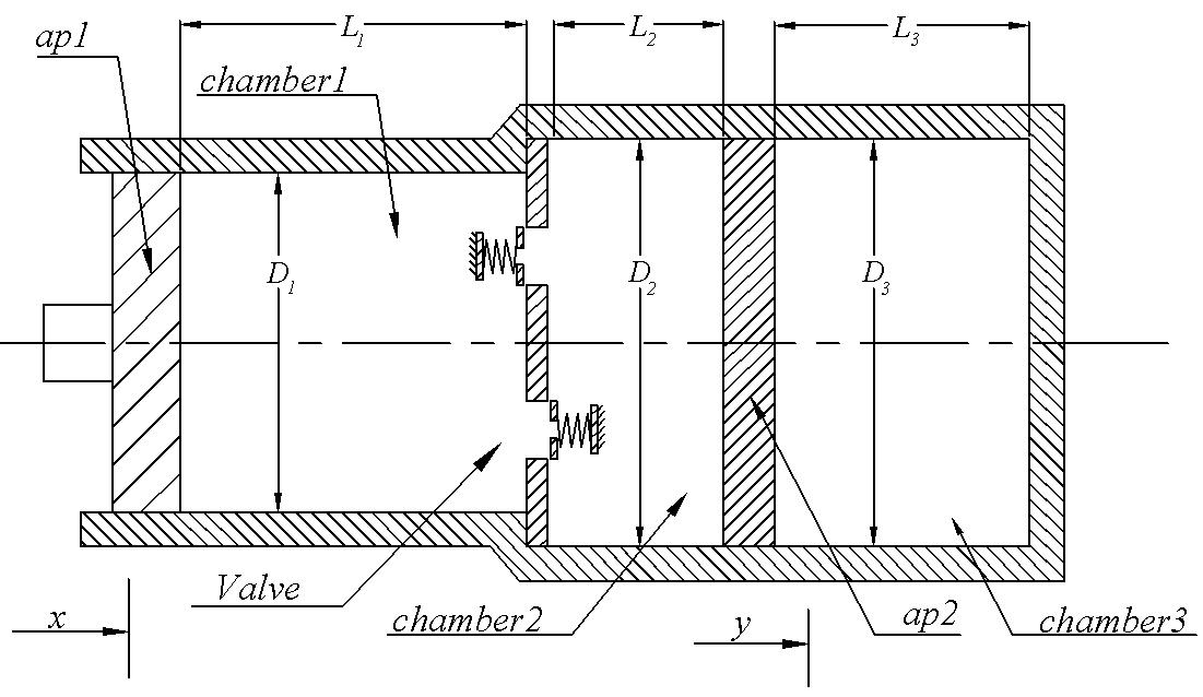
In this section a model of the hydro-gas suspension unit is developed. A diagram of the key elements of the device is shown in Figure 2.

Assumptions:

The main assumptions made when formulating the model are:

• Friction is neglected.
• Thermal effects caused by the heating of the oil as it passes through the valve are neglected.
• The mass of the floating piston is negligible (including the mass would result in high frequency dynamics, which causes problems for the model simulation).
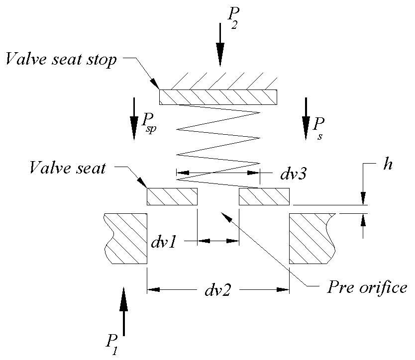
• The valve seat is assumed to be spring loaded with a simple pre-orifice on the seat (See Figure 4).
• The effective bulk modulus accounts for the compliance of the cylinder, compressibility of the fluid and compressibility of gaseous vapours present in the fluid.

Fundamental equations:

The equation of state for a liquid is given by [4]:

$\rho ={\rho }_o\left[1+\frac{1}{K_e}\left(P-P_o\right)\right]$ ()

In this equation, K_e is the effective bulk modulus, ρ_o and ρ are densities before and after a change in pressure of P_o to P.

The reversible adiabatic relationship for ideal gases is given by:

${\text{PV}}^{\gamma }=P_o{V}_o^{\gamma }$ ()

where, V_o and V are volumes before and after compression respectively, and γ is the adiabatic index, which is taken as 1.4 in this study.

Consider the model of the hydro-gas suspension unit shown in Figure 2. The following equations can be written for chamber 1 [5]:

$V_1=V_{\text{10}}-\text{ap}1\text{.}x$ ()

$m_1=m_{\text{10}}-\int {\dot{m}}_v\text{.}\text{dt}$ ()

${\rho }_1=\frac{m_1}{V_1}$ ()

Hence from Equation (1):

$P_1=K_e\left(\frac{{\rho }_1}{{\rho }_o}-1\right)+P_o$ ()

For chamber 2 [5]:

()

$m_2=m_{\text{20}}+\int {\dot{m}}_v\text{.}\text{dt}$ ()

${\rho }_2=\frac{m_2}{V_2}$ ()

Using Equation (1):

$P_2=K_e\left(\frac{{\rho }_2}{{\rho }_o}-1\right)+P_o$ ()

For chamber 3, having assumed that the mass of the floating piston is negligible:

$P_2=P_3$ ()

$V_3=V_{\text{30}}-\text{ap}2\text{.}y$ ()

$V_3^{\gamma }=\frac{P_o{V}_o^{\gamma }}{P_3}$ ()

Substituting Equations (10) and (13) into Equation (11) gives:

$K_e\left(\frac{{\rho }_2}{{\rho }_o}-1\right)+P_o=\frac{P_o{V}_o^{\gamma }}{V_3^{\gamma }}$

$$$\therefore m_2=V_2{\rho }_o\left[\frac{1}{K_e}\left(\frac{P_o{V}_o^{\gamma }}{V_3^{\gamma }}-P_o\right)+1\right]$ ()

Substituting Equations (7) and (14) into Equation (8) gives:

$\int {\dot{m}}_v\text{.}\text{dt}+m_{\text{20}}=V_2{\rho }_o\left[\frac{1}{K_e}\left(\frac{P_o{V}_o^{\gamma }}{(V_{\text{30}}-\text{ap}2\text{.}y{)}^{\gamma }}-P_o\right)+1\right]$ ()

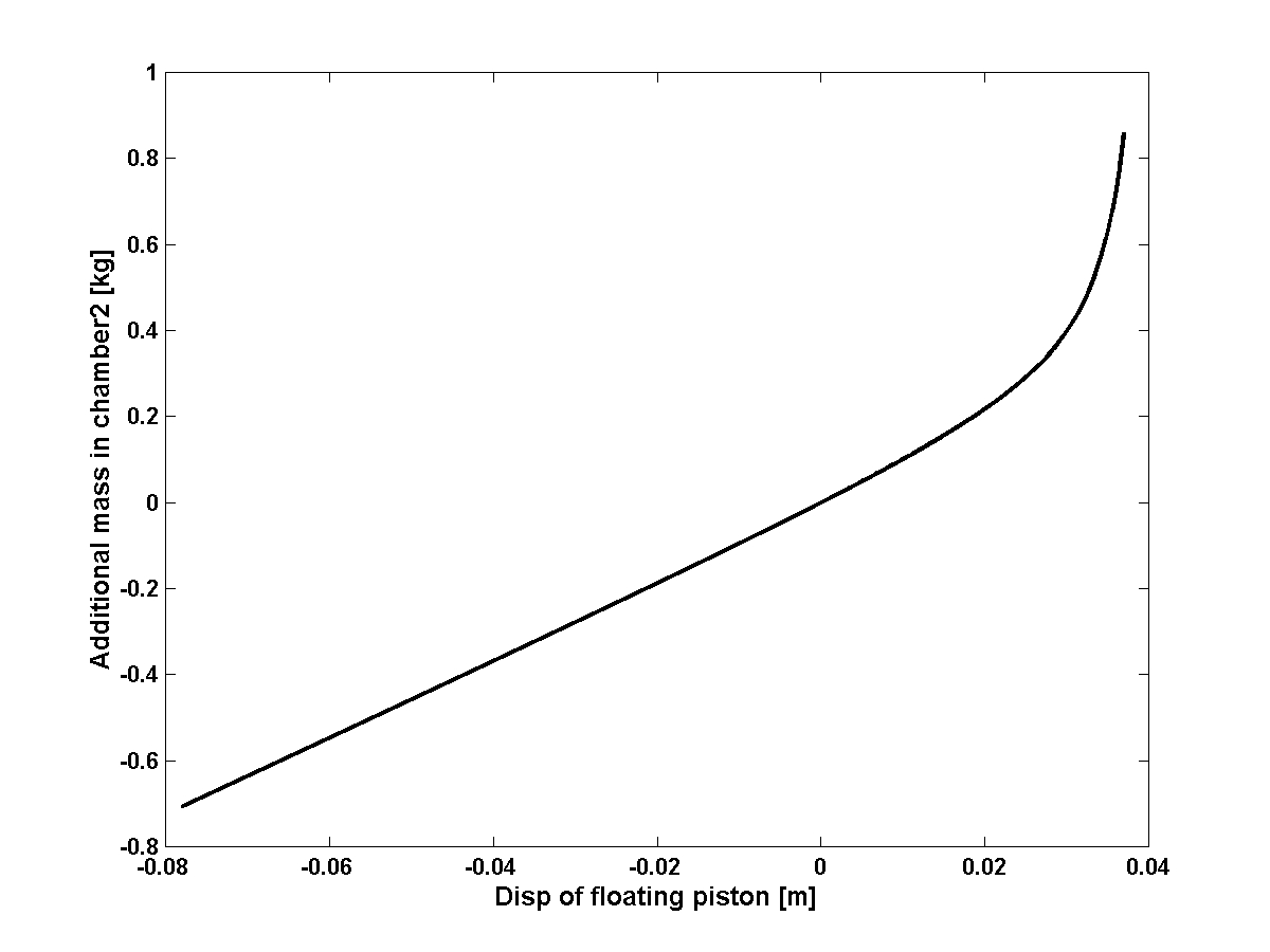
An algebraic loop was formed while simulating the above set of equations, which caused problems for the simulation. To overcome this, the relationship between $\int {\dot{m}}_v\text{.}\text{dt}$ and y, Equation (15), is obtained for a range of displacements (y) of the floating piston and incorporated into the model as a lookup table. In effect the problem has been reversed (consider a point (a,b) on the curve in graph shown in Figure 3) and posed as follows: if the floating piston has moved by an amount a, then fluid mass of amount b must have entered into chamber 2. It can be seen from the graph that the effect of gas pressure (steep increase in slope) comes into play as the floating piston moves towards the gas end (positive values) of the HSU and remain almost linear otherwise.

To incorporate the effect of the valve seat opening with pressure difference across them [6,7], the following assumptions are made:

• For the purpose of mathematical model, two valves, one for each direction of flow are depicted.
• The valves are assumed to be ideal non-return valves.
• There is no damping of the valve seat.
• The valve seat is considered massless (that is, no dynamics in the valve),
• The valve opening is only dependent on the pressure difference in chambers 1 and 2.

Figure 4 shows a cross section of one of the valves controlling flow from chamber 1 to 2. Pressure in chamber 2, P₂ assisted by the spring pressure P_s and spring overload pressure, P_sp in overcoming the pressure in chamber 1, P₁. When the pressure P₁ exceeds P_v, the sum of pressures P₂, P_s and P_sp, the valve seat lifts upwards thus changing the orifice area and hence the damping in the system.

$\sum P_v=0\Rightarrow \frac{\text{kh}}{\frac{\pi }{4}(\text{dv}{3}^2-\text{dv}{1}^2)}+P_2+P_{\text{sp}}=P_1$ ()

Here, k is the spring rate and h is the height to which the valve is lifted.

A spring-loaded ball (not shown in figure) works as a non-return valve, allowing fluid to flow through the pre-orifice in one direction only. Hence on rearranging Equation (16), we have:

$h=\frac{(\Delta P-P_{\text{sp}})\frac{\pi }{4}(\text{dv}{3}^2-\text{dv}{1}^2)}{k},\Delta P\ge P_{\text{sp}};h=0,\Delta P<P_{\text{sp}};$ ()

$\Delta P=(P_1-P_2)$ ()

where ΔP is the pressure difference across the valve. The resistance offered to flow by an orifice is given by [4]:

$R_v=\frac{1}{C_d{a}_v}\sqrt{\frac{1-{\left(\frac{a_v}{\text{ap}1}\right)}^2}{2{\rho }_o}}$ ()

here: $a_v=\frac{\pi }{4}\text{dv}{1}^2+\pi \text{.}h\text{.}\text{dv}2$, and

R_v is the valve resistance, C_d is the discharge coefficient, and a_v is the effective orifice area of the valve.

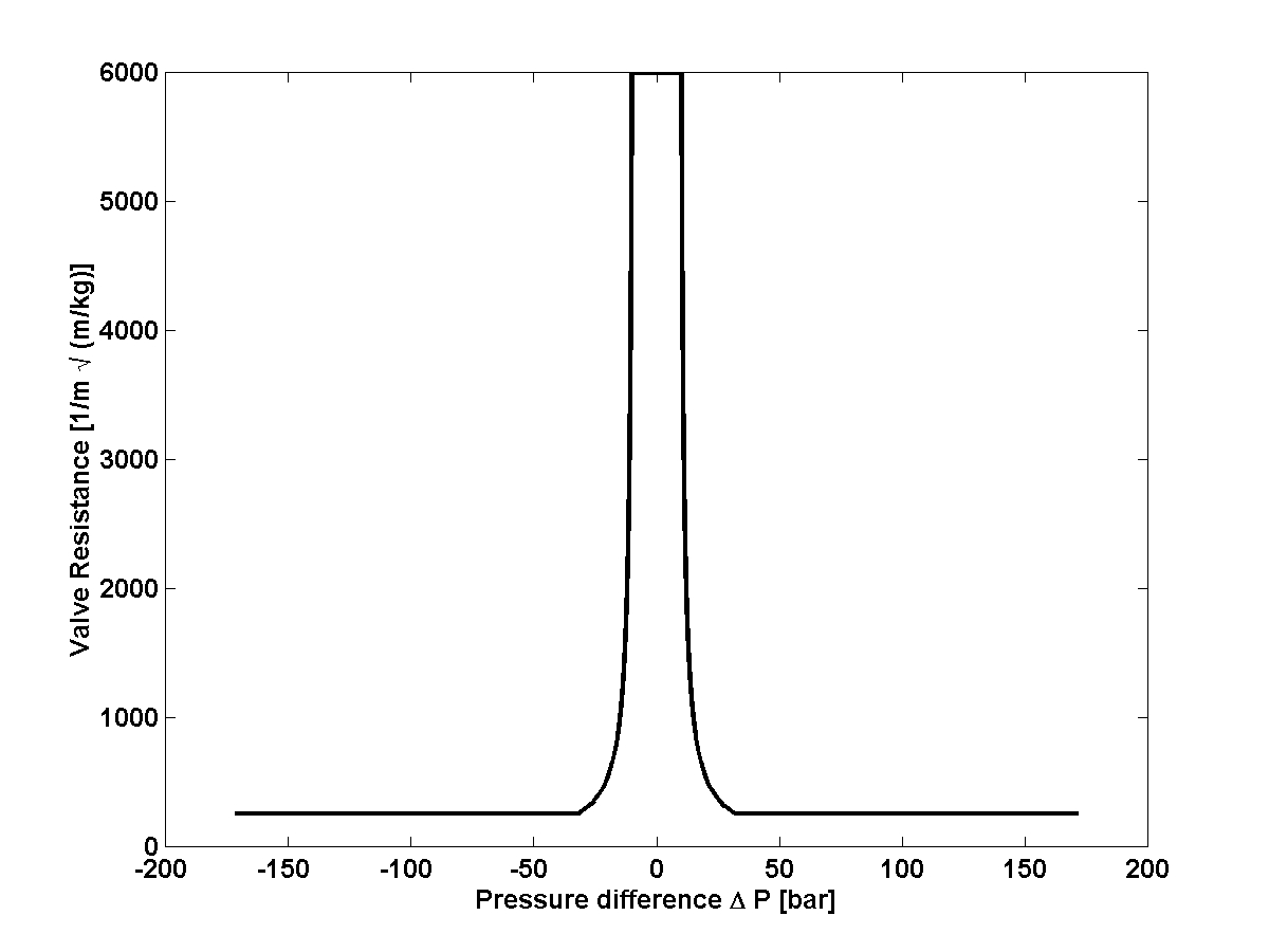
To facilitate programming, the valve resistance was calculated using Equation (19) for the complete range of pressure differences, ΔP, prior to the simulation and incorporated into the model as a lookup table. A plot of the variation of R_v with respect to ΔP is shown in Figure 5. It can be seen from the graph that R_v is high for small ΔP due to the pre-orifice (since ΔP < P_sp). As ΔP increases beyond P_sp, value of R_v falls till the valve hits the stop at maximum value of h, after which the resistance remains constant.

HSU simulation

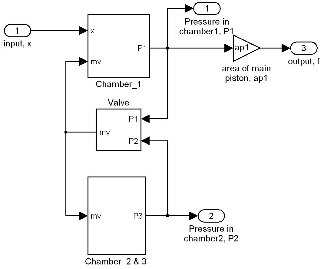
Figure 6 illustrates the top-level simulation diagram for Simulink.

The HSU model requires the main piston displacement as an input. Figure 7 shows the variation of suspension force with main piston displacement for pre-orifice diameters of 1 mm and 8 mm. The variation of force with frequency of excitation increasing from 1 Hz to 9 Hz for constant pre-orifice diameter is also shown.

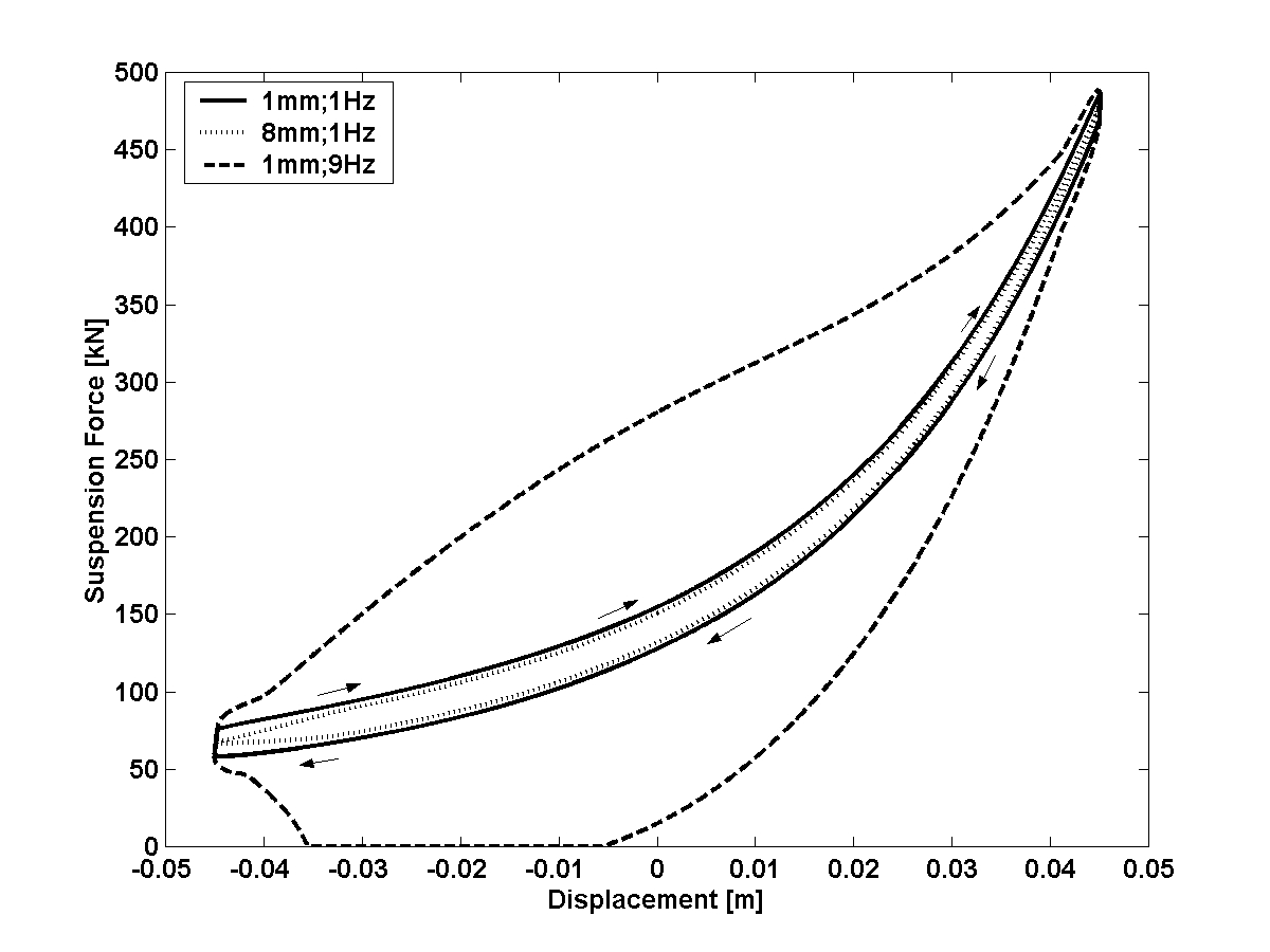
One of the salient features of this type of suspension is the capability of providing a rising spring rate that is, an increase in stiffness (slope of the curve) with increasing compression of gas, as can be seen in this graph. However, unlike a simple gas spring, the forward and return paths of the suspension force do not overlap. The direction of the arrows shows the trace followed by the force. The curve forms a loop, thus indicating hysterisis due to damping. The area within the loop is the energy dissipated due to damping.

The solid and dotted lines (the inner loop on Figure 7) show the variation of suspension force with actuating piston displacement for change in the damper valve orifice from 1 mm to 8 mm at 1 Hz. As the orifice decreases from 8 mm to 1 mm, the area within the loop increases indicating an increase in the energy dissipated and hence the damping in the system.

The solid and dashed dot lines (the outer loop on Figure 7) show the variation of suspension force with actuating piston for change in frequency of excitation. As the frequency of excitation increases from 1 Hz to 9 Hz with the 1-mm orifice diameter, the area of the loop formed also increases, with a corresponding increase in the damping. The shape of the curve deviates further from the previous curve in the middle region (low displacement—high velocity) than it does in the extremes (high displacement—low velocity). This is as expected, since damping is directly dependent on the velocity and hence the flow of fluid through the orifice.

Additionally, as the frequency of excitation increases while keeping the amplitude constant, a region is formed during the return stroke (piston moving away from the damper orifice) where the suspension force becomes almost zero. This phenomenon is due to the pressure within chamber 1 approaching zero and cavitation occurring, this is when the velocity of the piston is so large that fluid does not have enough time to pass through the orifice from chamber 2 into chamber 1. It can be noted that, as the orifice diameter decreases or the frequency increases, cavitation starts to occur more readily.

In reality, during the forward stroke, the piston forces the fluid through the damper orifice, while on the return stroke, it is the gas, which is under pressure that forces the fluid through the orifice. Hence the piston moves away at the pace decided by the amount of fluid that can pass through the orifice, whereas in the model the piston is reducing the pressure in the fluid causing the cavitation phenomenon. Hence, this phenomenon is unlikely to occur in reality.

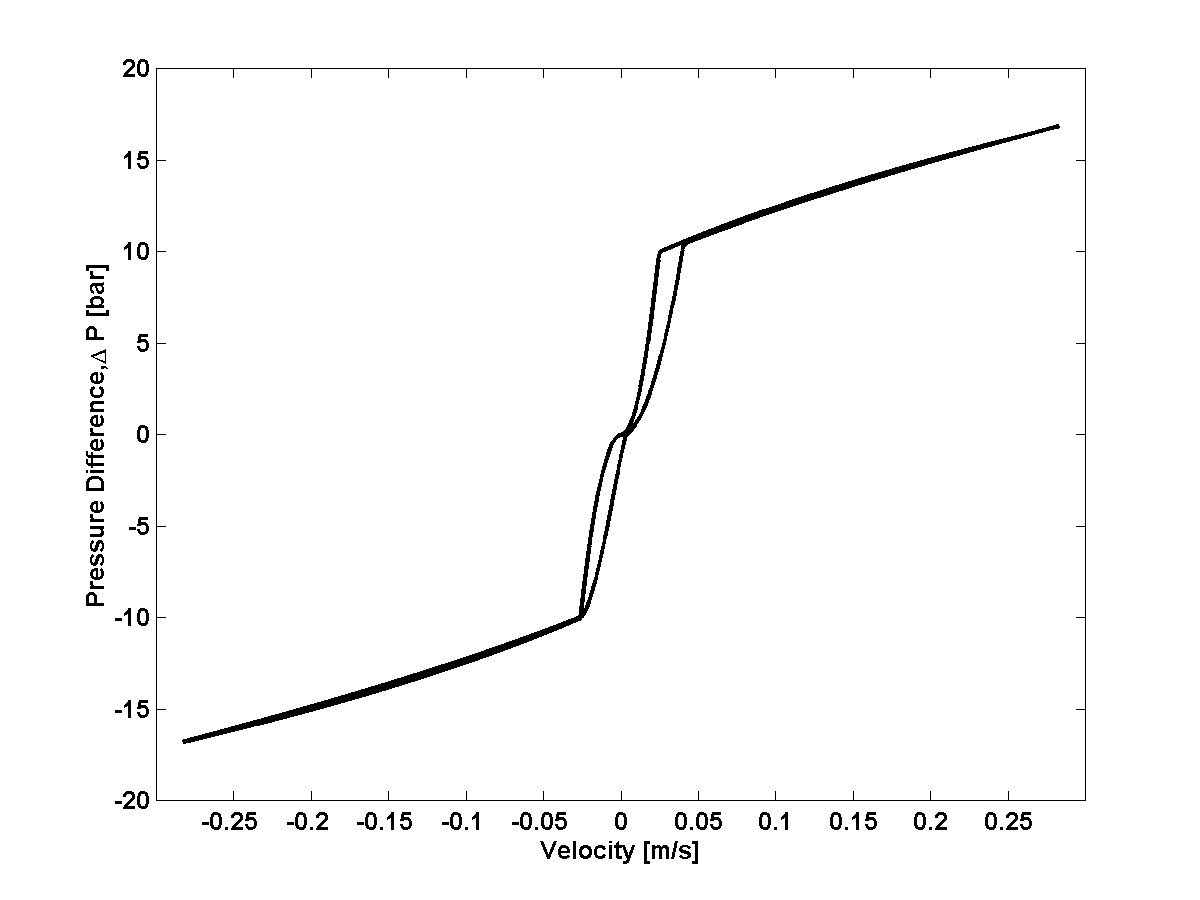
Figure 8 shows the variation of the ΔP with the velocity of main piston for a frequency input of 1 Hz. It can be seen in the graph that there are two separate parts to the curve. It was described above that damper assembly consists of a pre-orifice and a valve seat whose opening depends on the pressure difference across it. At lower velocities (+/– 0.03 m/s), the curve is parabolic which is due to the damper pre-orifice only, prior to opening of the valve seat. At higher velocities, the pressure difference between chambers 1 and 2 exceeds the preload of the spring retaining the valve in its seat and the valve starts to open. When the valve opens, the orifice area is increased, this leads to a nearly linear variation of pressure difference with the velocity of the piston. The rate of change of pressure difference, which is initially high, reduces in this region.

Trailing arm kinematics

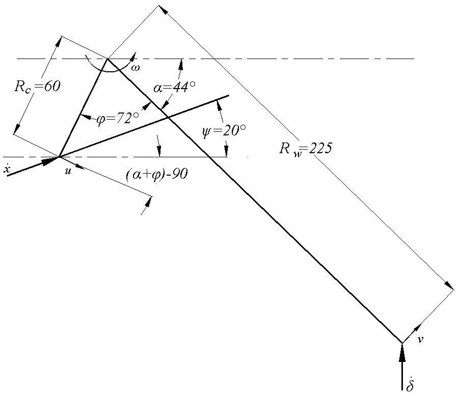
The geometry of the trailing arm is shown in Figure 9, for a tracked military vehicle along with typical dimensions for a Challenger 2 main battle tank. The suspension is drawn at the rebound position. A relationship between the wheel travel δ and the corresponding piston travel x of the HSU is to be obtained.

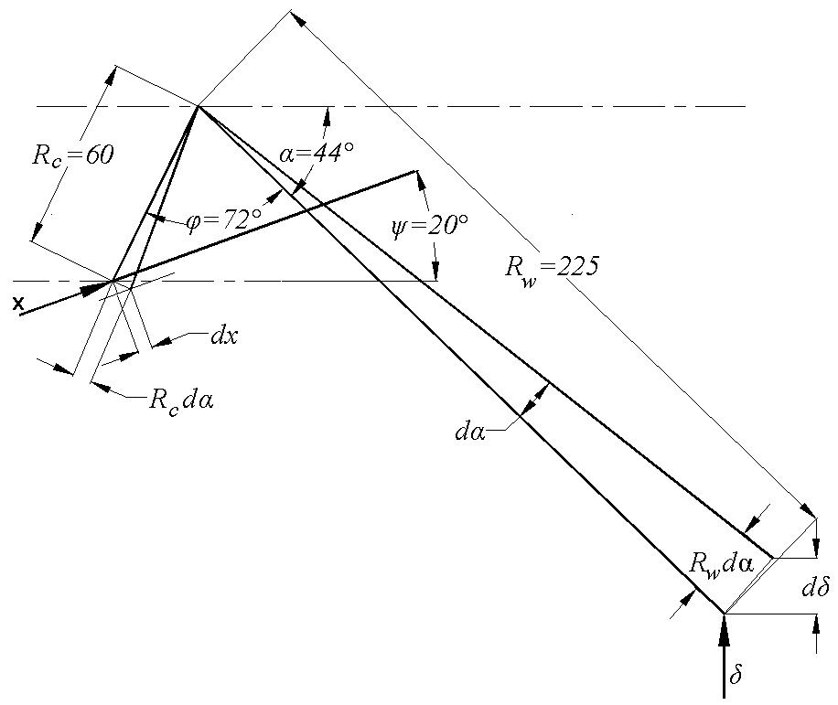
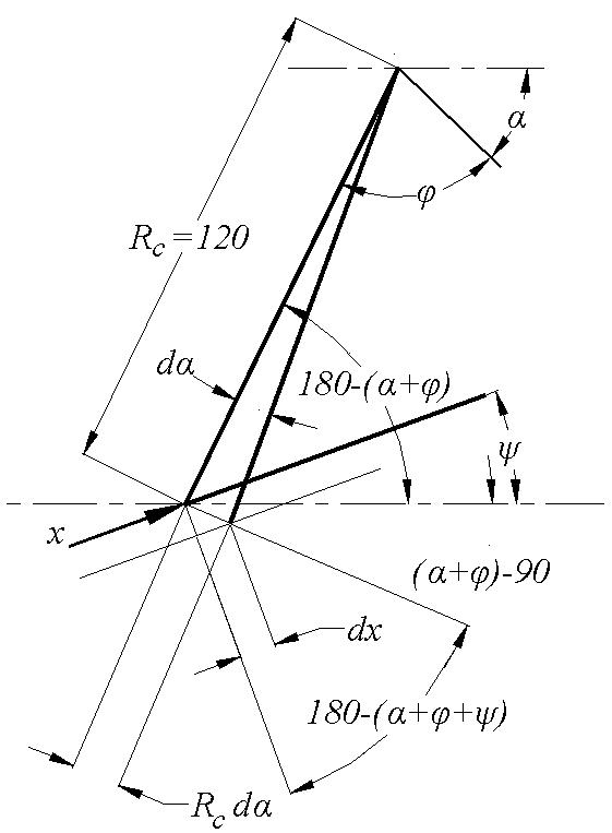
An increment of wheel travel towards bump dδ produces a corresponding piston travel dx along with the axle arm angle dα as shown in Figure 9. Figure 10 shows the crank end in greater detail.

$d\delta =R_{w}d\alpha \text{sin}(\text{90}-\alpha )$ ()

Displacement

$\text{dx}=R_{c}d\alpha \text{sin}[\text{180}-(\alpha +\phi +\psi \left)\right]$ ()

Eliminating dα from Equations (19) and (20), we have:

$\text{dx}=\frac{R_c\text{sin}[\text{180}-(\alpha +\phi +\psi \left)\right]}{R_w\text{sin}(\text{90}-\alpha )}d\delta$ ()

Velocity

Here the relation between the rate of wheel travel and the rate of piston travel is obtained. It is assumed that the trailing arm is rotating with an angular velocity ω rad/s. Then, the linear velocity ν perpendicular to the axle arm is given by:

$v=R_w\omega$ ()

and in the vertical direction:

$\dot{z}=v\text{cos}\left(\alpha \right)=R_w\omega \text{cos}\left(\alpha \right)$ ()

Similarly, at the crank end, the linear velocity, u, perpendicular to the crank is given by:

$u=R_c\omega$ ()

and in the direction of travel of the suspension piston by:

$\dot{x}=u\text{c}\text{o}\text{s}(\alpha +\phi +\psi -\text{90})=R_c\omega \text{c}\text{o}\text{s}(\alpha +\phi +\psi -\text{90})$ ()

Eliminating ω from the above two equations we have:

$\dot{x}=\frac{R_c\text{cos}(\alpha +\phi +\psi -\text{90})}{R_w\text{cos}\left(\alpha \right)}\dot{\delta }$ ()

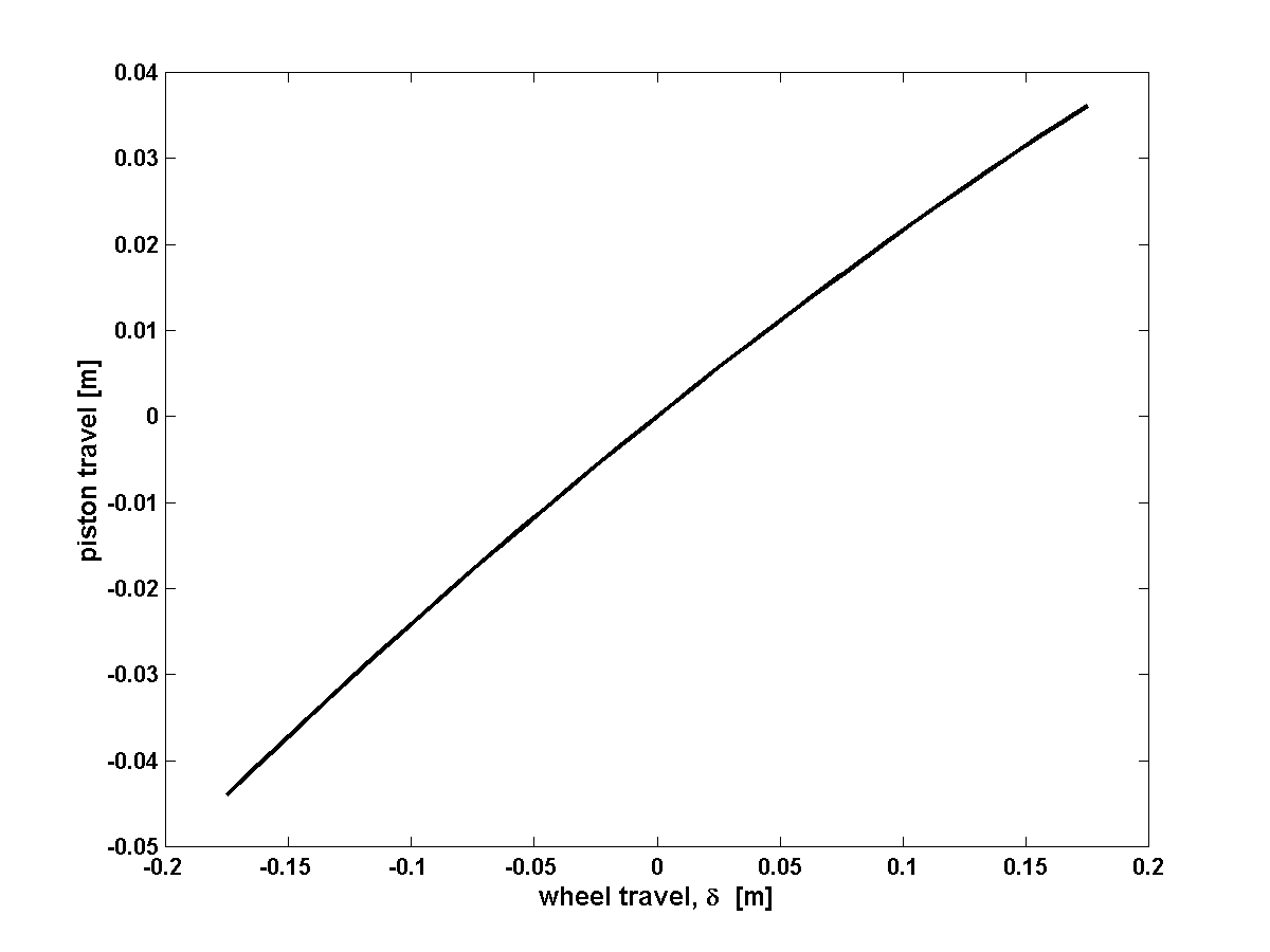
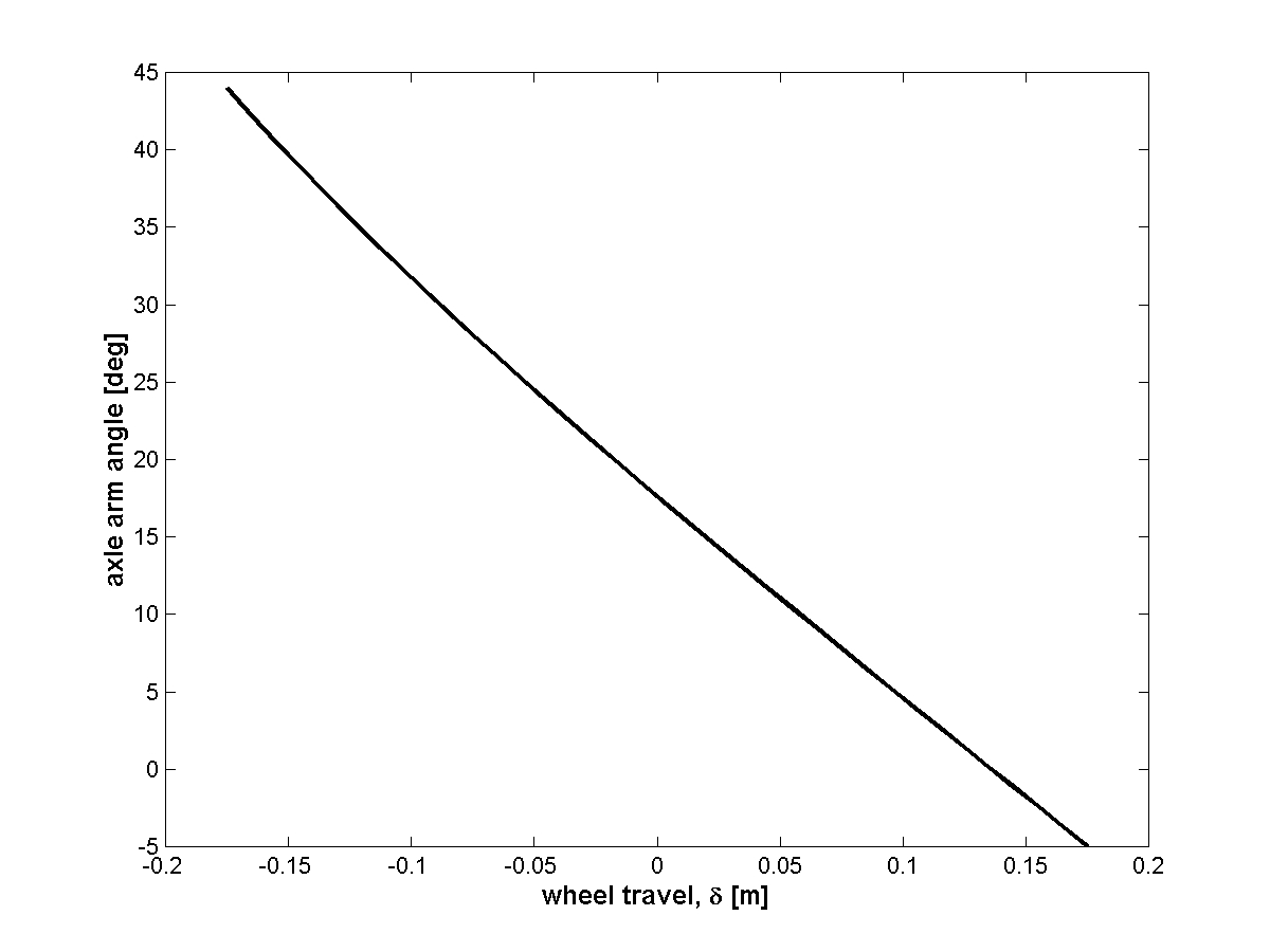
Figure 12 shows the relationship between the road wheel travel and piston travel of the hydro-gas suspension unit. The rotation of the trailing arm with wheel travel is shown in Figure 13. Both of these graphs are incorporated into the model as look-up tables. It could, however, be argued that they could have been linearised about the nominal ride height of the vehicle.

Six wheel station vehicle model:

In this section the model of the HSU is incorporated into a six-wheel station tracked vehicle model, a diagram of which is shown in Figure 14. Here the vehicle body is assumed to be perfectly rigid and having two degrees of freedom—namely, pitch, θ and bounce, z_s. The sprung mass of the body is m_s and its moment of inertia about the centre of mass is I_s. For each suspension station, the suspension force is denoted by f_si, unsprung mass by m_ui, road wheel stiffness by k_ui and damping by c_ui, where subscript i varies from 1 to 6.

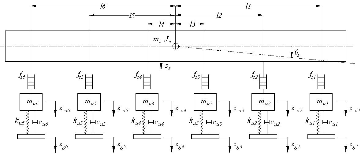
The bounce equation of motion for the HSU in tension is given by:

$m_s{\ddot{z}}_s=m_{s}g+f_{s1}+f_{s2}+f_{s3}+f_{s4}+f_{s5}+f_{s6}$ ()

where g is the acceleration due to gravity. The forces in the hydro-gas suspension units are functions of the displacements across them, these are determined from the motions of the body and unsprung masses and the kinematic relationships derived earlier.

Similarly the pitch equation of motion is given by:

$I_s{\ddot{\theta }}_s=l_{1\text{.}}{f}_{s1}+l_{2\text{.}}{f}_{s2}+l_{3\text{.}}{f}_{s3}+l_{4\text{.}}{f}_{s4}+l_{5\text{.}}{f}_{s5}+l_{6\text{.}}{f}_{s6}$ ()

The equation of motion for the unsprung masses is given in Equation (30), in which it has been assumed that the road wheel is in compression;

$m_{\text{ui}}{\ddot{z}}_{\text{ui}}=-f_{\text{si}}-k_{\text{ui}}(z_{\text{ui}}-z_{\text{gi}})-c_{\text{ui}}({\dot{z}}_{\text{ui}}-{\dot{z}}_{\text{gi}})+m_{\text{ui}}g$ ()

where subscript i varies from 1 to 6.

Vehicle simulation

In this part the results from the simulation of the vehicle, with hydro-gas suspension are presented and discussed. The vehicle is simulated crossing a piece of terrain, which starts at 0.1 Hz and ends at 30 Hz with a variable amplitude. The amplitude is selected to give a constant velocity profile and is commonly used in vehicle dynamics investigations. The range of frequencies has been selected to encompass those of the body and road wheels and is typically that used for ride assessment of vehicles.

In reality the ground input is random. However, it was found that using the model for suspension optimisation studies, with random terrain, caused problems for the optimization routine (the optimization results are not presented in this work), hence a constant velocity input was used.

The weighted rms body acceleration obtained at the driver’s station against orifice diameter is show in Figure 15. The driver’s station is located 2 m in front of the centre of mass of the vehicle. The acceleration data has been weighted using the filter given in ISO 2631 [10] for vertical motion.

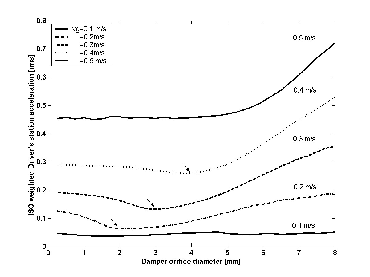
For the three ground inputs 0.2, 0.3 and 0.4 m/s (Figure 15), the body acceleration tends to reach a minimum value, which indicates that there is an optimum orifice diameter for these terrains (indicated by arrows). As the ground roughness increases, for these three plots, the point of optimum damping moves towards larger orifice diameters, hence less damping. It can be seen from the graph that for ground input velocity of 0.2 m/s a damper orifice diameter of 2 mm would be best, while for the 0.3 m/s case it is 3 mm and then 4 mm for 0.4 m/s.

As the ground velocity increases above 0.4 m/s, the curve gets flatter in the left region. This is to say that as the terrain becomes more and more rough, the damping required for the vehicle decreases to provide good ride performance. For instance when the ground input velocity gets to 0.5 m/s, the curve does not exhibit a minimum, which indicates that higher the ground input velocities, the larger the range of the damper setting which would provide the required ride performance.

As can be seen from the above graph, the optimum damper orifice diameter varies from 2 mm for 0.2 m/s to 4 mm for 0.4 m/s input. Hence as a first approximation, we could arrive at a reasonable ‘best value’ of 3-mm orifice diameter for good ride performance over the range of velocity inputs considered.

Conclusions

A mathematical model for the hydro-gas suspension unit has been developed and simulated using Matlab and Simulink Software. This model incorporates compressibility of fluid and spring-loaded damper valve in its formulation.

A method of using lookup tables has been proposed for overcoming the problem encountered with an algebraic loop while calculating the flow through the damper valve during simulation.

The variation of different parameters of the hydro-gas suspension unit (namely, suspension force and pressure difference across damper valve) for changes in amplitude and frequency of actuation has been shown. In the process, the cavitation phenomenon has been demonstrated. However, this phenomenon is unlikely to occur in reality.

The model thus developed has been mounted into a six-wheel station tracked vehicle model and simulated for known inputs. Optimisation of the ride characteristics with respect to the suspension damping has been carried out for a variety of constant velocity terrain input in the frequency range between 0.1 to 30 Hz by varying the damper orifice diameter.

It has been shown that a damper orifice diameter of 3 mm is a good compromise for ride performance over both smooth and rough terrain.

References

Authors

David Purdy is currently a senior lecturer for Cranfield University at the Royal Military College of Science in the Engineering Systems Department. His current research interests are military vehicle dynamics and weapon control systems.

J. Rajesh Kumar is a scientist working on tracked military vehicles with Combat Vehicles Research and Development Establishment, Ministry of Defence, DRDO, India. Currently he is studying for an MSc in Military Vehicle Technology at the Royal Military College of Science.

References

J.Y. Wong, Theory of Ground Vehicles, John Wiley & Sons Inc, Third Edition, 2001.
B. Maclaurin, “Progress in British Tracked Vehicle Suspension Systems”, SAE Technical Paper Series, 1983.
D. Karnopp, “Theoretical Limitations of Active Vehicle Suspensions”, Vehicle System Dynamics, Vol. 15, pp. 41–54, 1986.
H.E. Merritt, Hydraulic Control Systems, Wiley, New York, 1967.
D.J. Purdy, “Theoretical and Experimental Investigation into an Adjustable Automotive Damper”, Journal of Automobile Engineering (Part D), Vol. 214, pp. 265–283, 2000.
R. Karadayi, and G.Y. Masada, “Nonlinear Shock Absorber Model”,<strong> </strong>AMD (Symposia Series) (American Society of Mechanical Engineers, Applied Mechanics Division), Vol. 80, pp. 149–165, 1986.
C. Surace, K. Worden, and G.R. Tomlinson, “On the Non-Linear Characteristics of Automotive Shock Absorbers”, Proceedings of the Institution of Mechanical Engineers, Part D: Journal of Automobile Engineering, Vol. 206, No. 1, pp. 1–16, 1992.
“Dunloride Suspension System Suitable for Tracked Vehicles in 30–40 Tonne Weight Class”, Jane’s online.
Using Matlab—Simulink and Control System Toolbox, The Mathworks Inc.
“Guide For Evaluating The Human Response To Whole Body Vibration”, International Standard ISO 2631 Part 1, 4 & 5.