
Volume 7, Number 1, March 2004
Handling of Tracked Vehicles at Low Speed
- 1 Both authors are with: Engineering Systems Department, Royal Military College of Science, Shrivenham, Swindon, Wiltshire, SN6 8LA, United Kingdom.
Abstract
Determining the handling characteristics of tracked vehicles is significantly more complex than wheeled vehicles. This is because of the non-linear behaviour of the interaction between the tracks and ground during turning. In many cases a full dynamics model of the steering of a tracked vehicle is too complex and time consuming to generate and gives little or no insight into the mechanics of skid steer. This is especially true during the initial design phase, or the examination of a modification, when the designer needs a method, which allows the trade offs to be examined quickly. The work presented here is based on the method used at the Royal Military College of Science (RMCS) to teach the fundamentals of tracked vehicle steering and is suitable for low speed predictions only. Comparison of the method with experimental data shows that the radius of turn is determined with reasonable accuracy but only an upper bound is put on the sprocket torque. Modifications of this technique to include side force generation have been used successfully elsewhere to determine the behaviour of half-tracks and articulated track vehicles.
Nomenclature
| a | Longitudinal acceleration |
|---|---|
| C | Semi track of vehicle |
| F | Friction force |
| g | Acceleration due to gravity |
| L | Semi-length of track on ground |
| M | Slew moment |
| n | Steer ratio |
| P | Power |
| R | Radius of turn |
| SF | Slip factor |
| SRR | Specific rolling resistance |
| T | Torque |
| v | Vehicle speed |
| X | Longitudinal force component |
| x | Distance along track |
| Y | Lateral force component |
| Z | Normal force component |
| β | Non-dimensional slip radius |
| δ | Small increment |
| µ | Coefficient of friction |
| θ | Angle defined in Figure 1 |
| Ω | Yaw rate of vehicle |
| ω | Angular speed |
| Superscript | |
| ′ | Non-dimensional track force or moment |
| Subscript | |
| e | Operating condition |
| g | Slope of terrain |
| i | Inner track |
| o | Outer track |
| s | Sprocket |
Introduction
The majority of military high-mobility tracked vehicles use skid steer for changing direction. To initiate a turn in a skid steer tracked vehicle, the sprockets are prescribed to rotate at different speeds. After a period of time the vehicle should settle down into a steady-state turn, in which the outer track sprocket is rotating faster than the inner. The ratio of the outer to the inner sprocket angular speed is called the steer ratio n and is analogous to the steer angle of the front wheels of a wheeled vehicle.
The prediction of the handling characteristics of skid-steer tracked vehicles is a relatively complex problem [1,2,3]. In many cases though, the objective is to understand the low-speed characteristics for an initial design investigation or modification to an existing vehicle. In these cases, the need is for a method which rapidly allows the designer to balance the conflicting requirements. The technique given in this paper allows this by permitting the solution to be produced by hand or by the construction of a suitable spreadsheet.
At the present time many sophisticated models are available for solving the handling problem of tracked vehicles [1–3]. These models require large amounts of computing power to generate the solutions and can detach the user from the underlying mechanics of skid steer. The work presented in this paper allows the user to obtain a fundamental understanding of skid steering and a way of checking the low speed response of more complex models.
A brief history of the techniques used to analyse skid steering is given by Purdy and Wormell [1]. The method presented here is a modification to that by Merritt and Steeds [4,5], for the case of a vehicle under a longitudinal load while executing a low-speed turn. The method developed does not require any iteration in its solution, which was a weakness in the original technique. The model developed is only suitable for low-speed operation involving lateral accelerations up to about 0.3g (3 m/s2) but this is normally sufficient for the majority of cases because of the limit oversteer behaviour of tracked vehicles [1]. The reason for this limitation is the exclusion of lateral acceleration from the model. The analysis allows the prediction of radius of turn, sprocket torque and power and the limiting conditions for steering to take place.
The method has been used for introductory courses on tracked vehicle steering at the Royal Military College of Science (RMCS) for many years. It has been successfully applied, with the addition of lateral force, to investigations on half-track and articulated track vehicles [6].
The sign convention and nomenclature used in this work follows that of the original [6].
Vehicle model
The vehicle model is built up in two stages in this section. Initially a single track is considered, which is sliding both longitudinally and laterally over the ground. Finally the whole vehicle is considered and combined with the track model. The main assumptions built into the model are:
- The ground is flat and rigid.
- The track to hull connection is laterally rigid.
- Uniform track loading.
- Isotropic Coulomb friction between the tracks and ground.
- The lateral acceleration is negligible and there is no weight transfer.
Track model
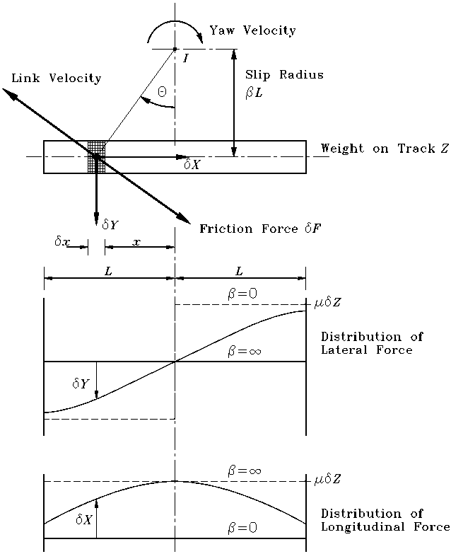
During a steady state turn, the track is sliding over the ground, a diagram of this is shown in Figure 1. In this diagram the sliding motion of the track can be viewed as rotating about an instantaneous centre at I. For zero resultant lateral force this centre of rotation is on a perpendicular from the plan centre of the track. The distance of the centre of rotation from the centre-line of the track is called the slip radius, which is given by βL where β is the non-dimensional slip radius [4].
The relationship between the slip radius and the longitudinal force and resisting moment can be obtained as follows. The friction force acting on an element of track, Figure 1, is given by:
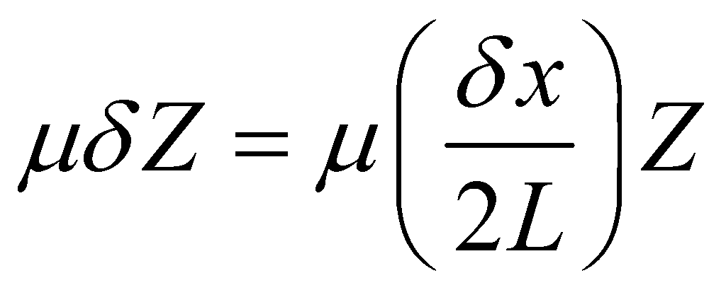
With its direction opposing the motion of the element across the surface of the ground. In this equation µ is the coefficient of friction, Z the weight on the track, δx is the length of an incremental section of track and L is the semi length of the track on the ground. The distribution of the longitudinal and lateral forces and their limiting values are shown in Figure 1.
Longitudinal force
The longitudinal friction force acting on the track is seen to be:
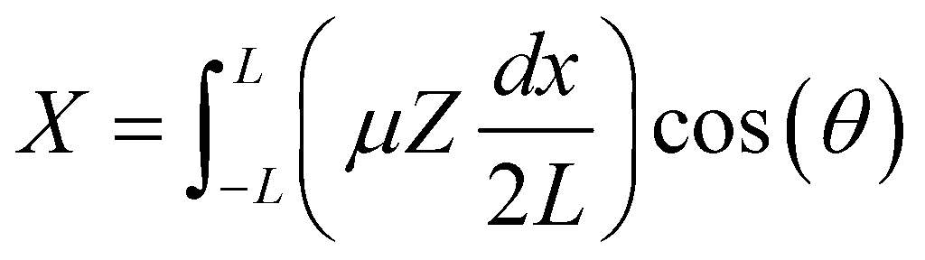
Where X is the force in the x-direction and θ is defined in Figure 1. Changing the variable from θ to x gives:
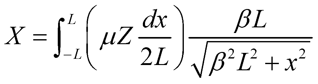
Integrating Equation (3) and making the substitution:
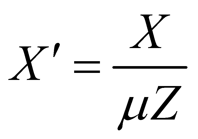
where is the non-dimensional longitudinal force gives:
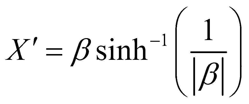
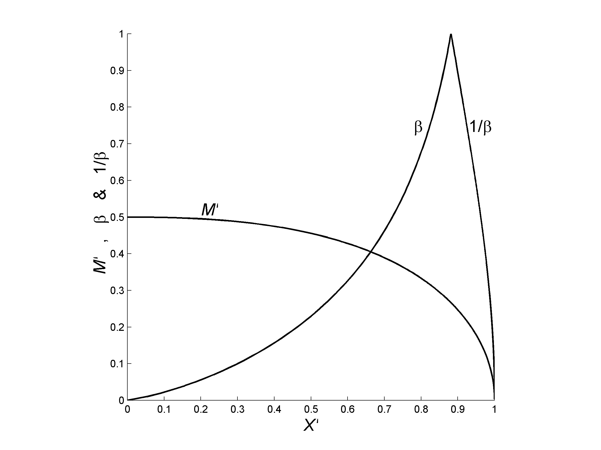
A plot of Equation (5) is given in Figure 2, which can be used to determine the slip radius given the longitudinal force on the track.
Lateral force
It can be shown, by performing the above analysis in the lateral direction, that the lateral force is zero. This is in accordance with the assumption that the centre of rotation is on the transverse centre line of the track.
Yaw moment
The yaw moment about the centre of the track is given, from Figure 1, by:
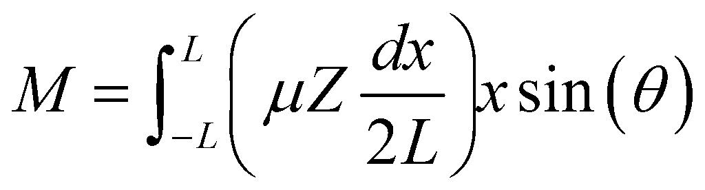
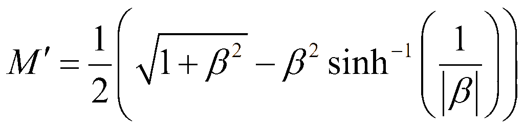
Where M is the resisting (slew) moment generated on the track, this equation can be integrated by a similar method to Equation (2), to give:
Where the non-dimensional slew moment:
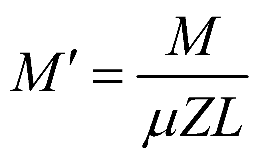
Equation (7) is also plotted on Figure 2.
Vehicle model
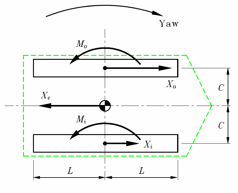
A free-body diagram for the complete vehicle is shown in Figure 3, where the longitudinal force Xe acting at the centre of mass will be used later to represent the effects of rolling resistance, gradient or acceleration, the operating condition. The inner track, subscript i, is the track closest to the centre of rotation of the vehicle and the outer track has a subscript o.
Longitudinal
The non-dimensional longitudinal equation for the vehicle, Figure 3, is given by:
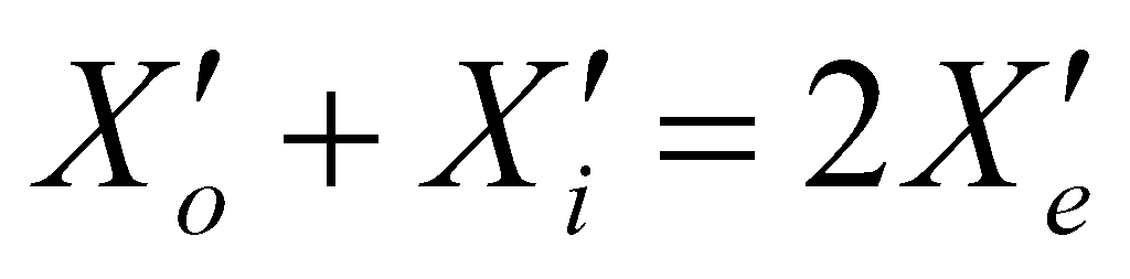
Where the non-dimensional operating condition:
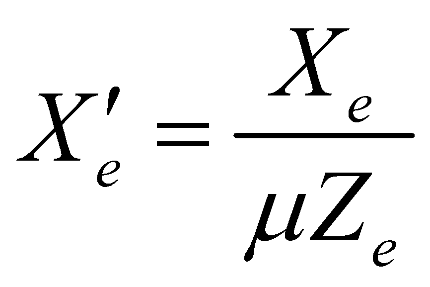
Equation (9), can be written as:

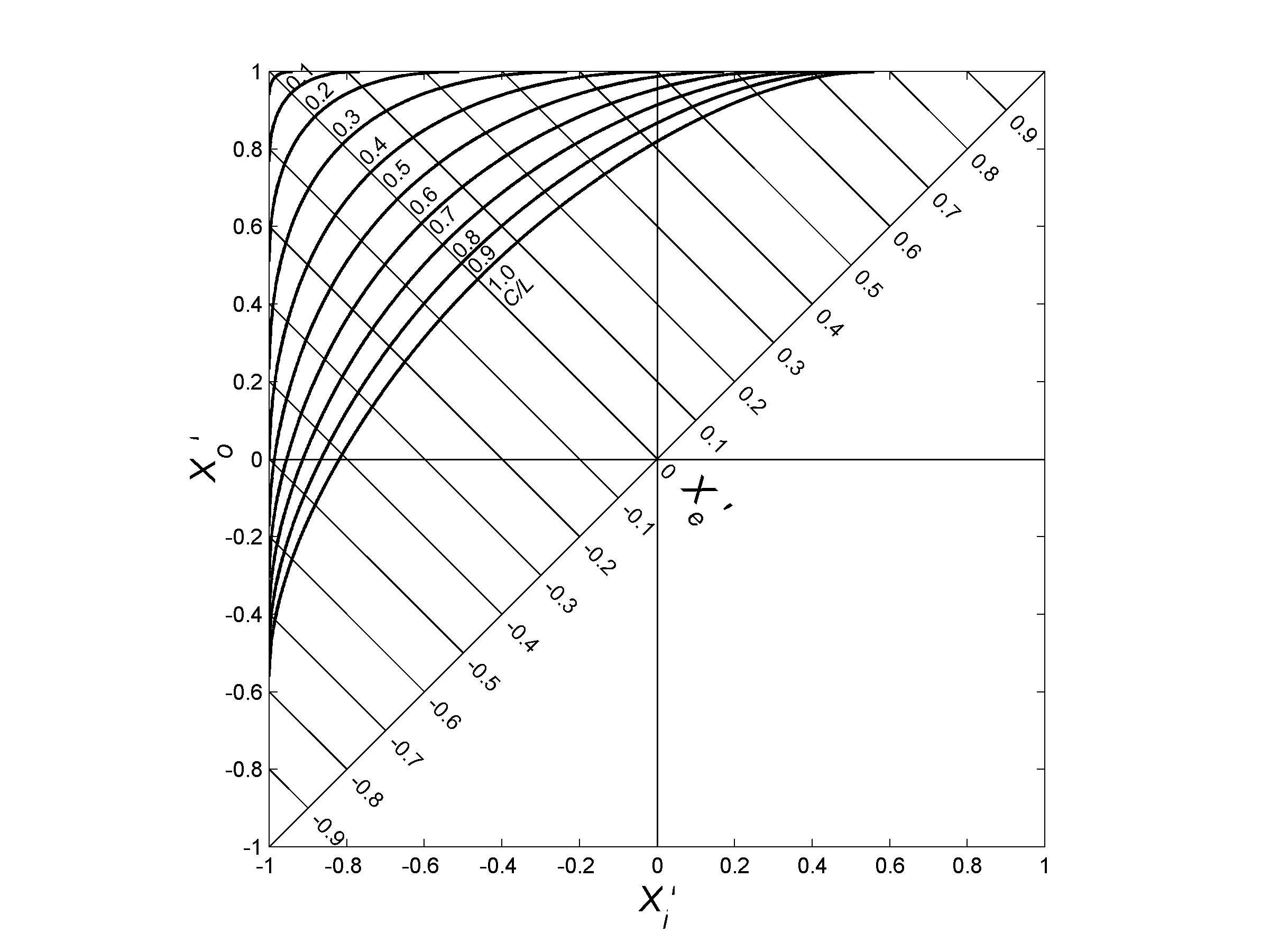
Thus the lines of constant operating condition will be straight lines with a slope of –1 on a plot of against , as shown in Figure 4.
Yaw
The non-dimensional equation for the yawing of the vehicle is given by:

Hence, using Equations (5) and (7); the vehicle ‘geometric ratio’ is:
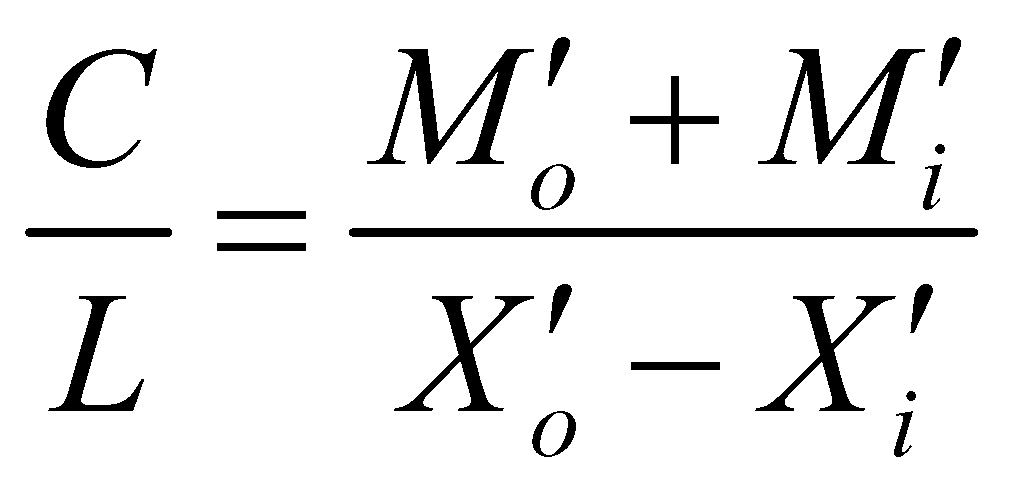
Given that is implicitly related to , Figure 2, this equation can be plotted, Figure 4, for different values of C/L. The plotting of this equation is complicated by its transcendental nature, which is greatly simplified by the use of a computer and appropriate software, in this case Matlab [7].
The pair of Equations (9) (or (11)) and (13), which are simultaneous in and , will yield the track forces necessary to achieve a turn for any given C/L ratio and operating condition . In practice this can be solved iteratively or more simply read off from the plot in Figure 4. In Figure 4, curves are given for the geometric ratio C/L from 0.1 to 1.0 and longitudinal force from –1.0 to 1.0, the practical range of interest for the geometric ratio is from 0.5 to 1.0.
The plot shown in Figure 4 shows how the longitudinal track forces vary with C/L ratio and operating condition . Without any longitudinal force the track forces are equal in magnitude but opposite in direction. The track force magnitude against C/L ratio is plotted in Figure 5, in this figure it can be seen that for very small C/L ratios, long thin vehicles, the track forces are approaching their limiting values.
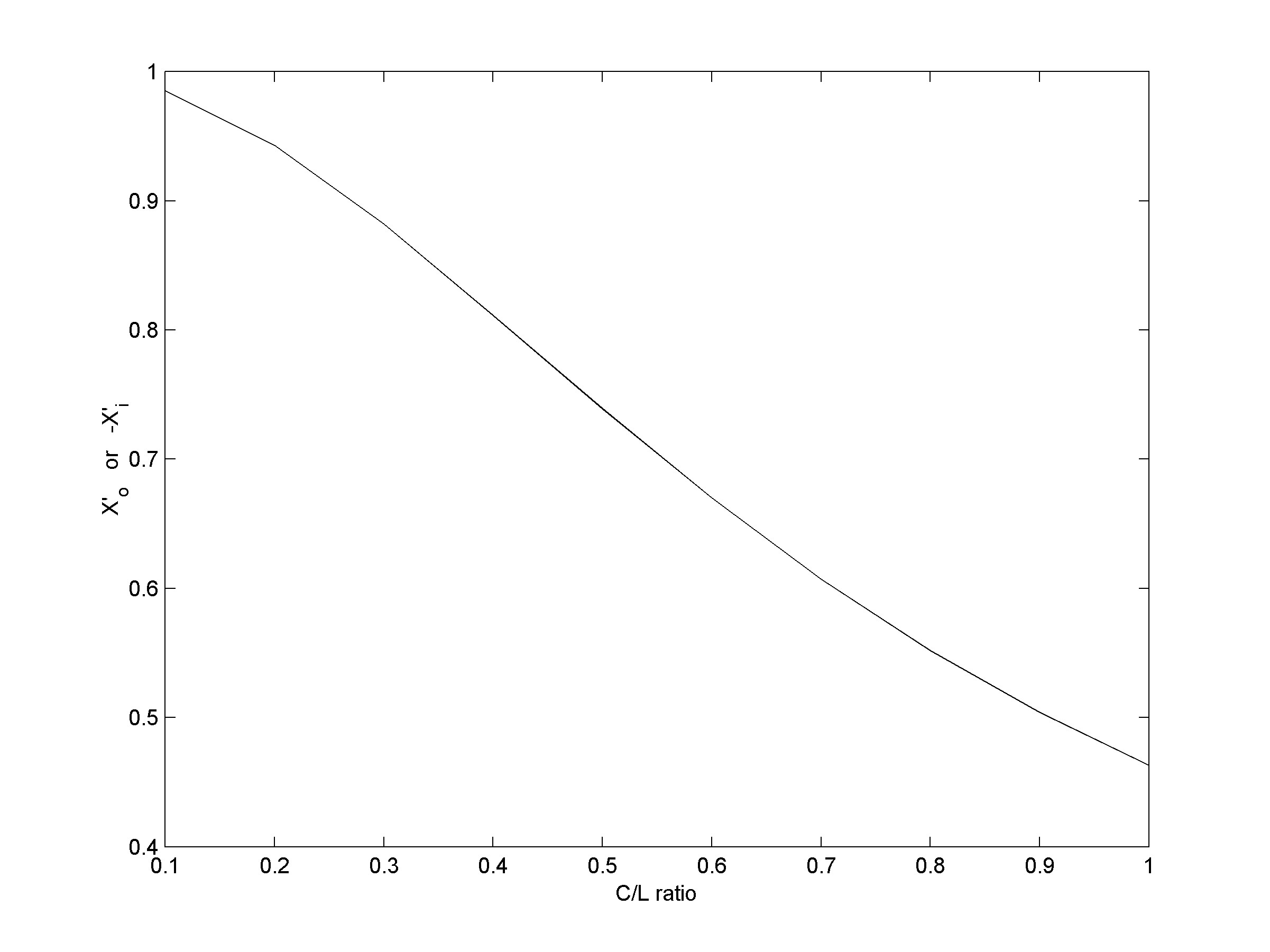
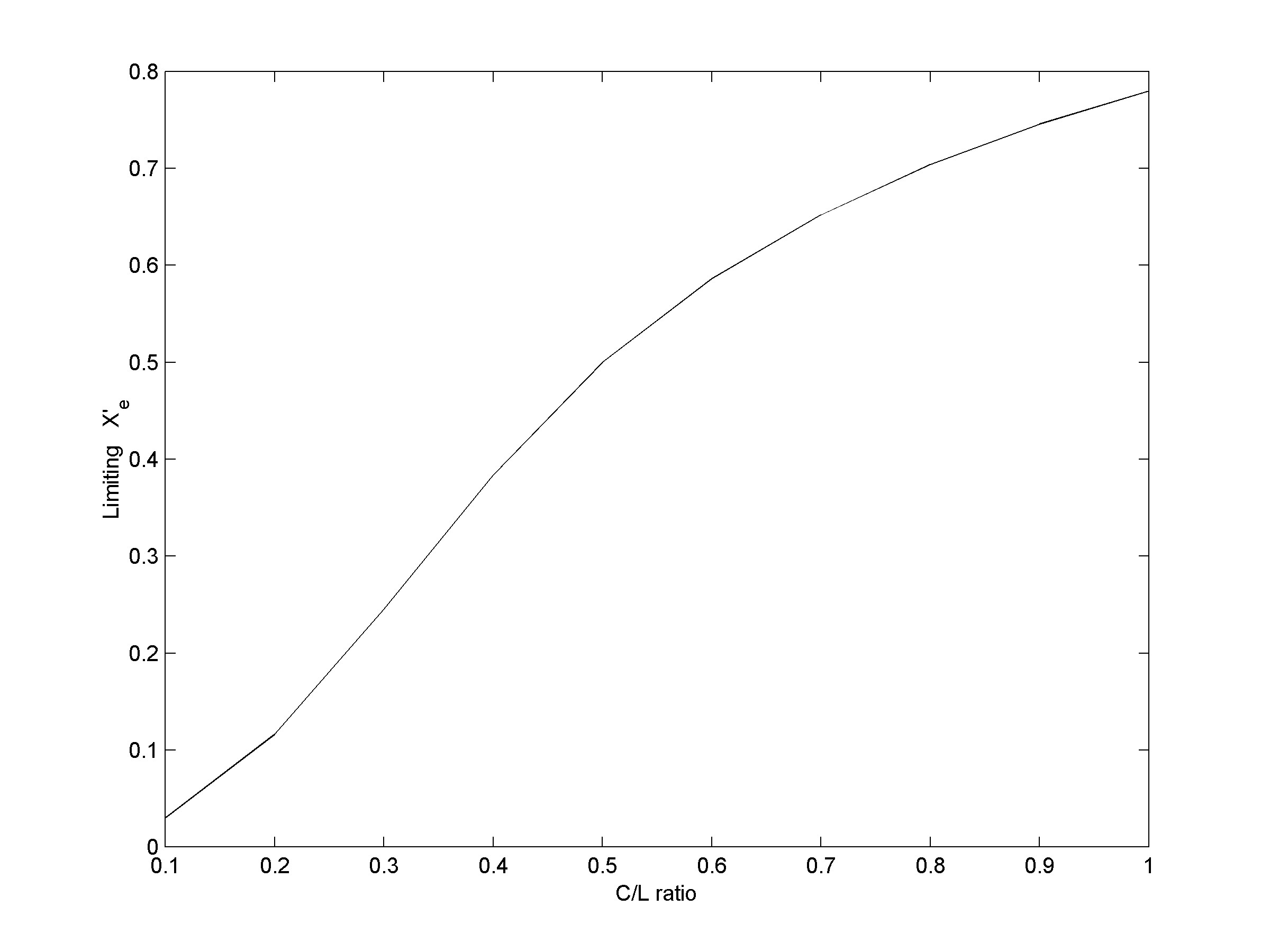
At the extremes of the diagram, Figure 4, the curves meet the and boundaries and the limit of available friction has been reached. Correspondingly, the slip radius β becomes infinite, as too does the radius of turn of the vehicle. A plot showing the limiting operating condition against C/L ratio is shown in Figure 6. In Figure 6 the plot shows that for small C/L ratios the vehicle is very close to the maximum longitudinal track forces that can be generated. Thus the vehicle is still able to steer but if any additional operating load were applied to it, it would rapidly become unsteerable.
Determining the non-dimensional longitudinal force x’e
Three cases are considered in this section—the effect of: gradient, rolling resistance and acceleration. The first of these is considered in detail while the results for the others are just quoted.
Gradient
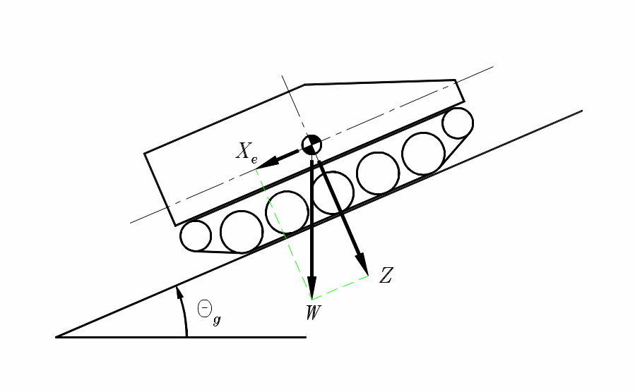
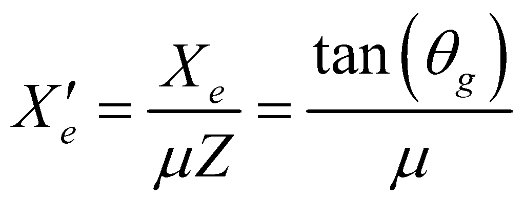
A diagram of a tracked vehicle climbing a slope of gradient θg is shown in Figure 7. In this figure the weight of the vehicle is W, which has been resolved into components along the slope and perpendicular to it. For this situation the operating condition is given by:
Rolling resistance and acceleration
Using the same approach for the Specific Rolling Resistance (SRR) results in an operating condition of:
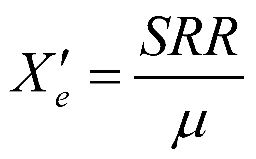
Where the SRR is the rolling resistance of the vehicle as a proportion of its weight.
The effect of acceleration on the operating condition is given by:
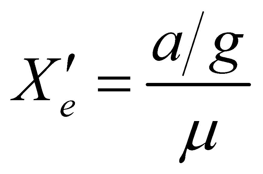
Where a is the acceleration of the vehicle and g is the acceleration due to gravity.
From the forgoing analysis the longitudinal track forces can be estimated, from which the sprocket torques can be determined, given the sprocket radius Rs:

Kinematics of skid steering
In this section a relationship is developed, which gives the radius of turn as a function of sprocket speed ratios, including the special case of turning on hard level ground. This analysis is then extended to encompass the engine slip factor and finally the power required.
Sprocket speed ratio
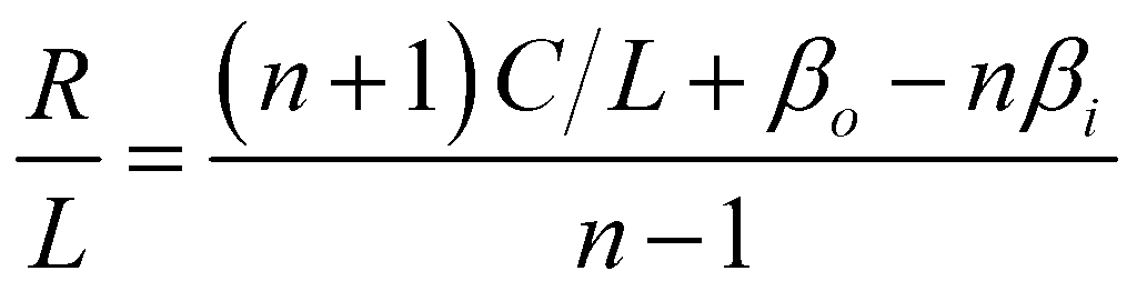
The angular speed of a sprocket is composed of two parts; that correspond to the required radius of turn in the absence of track slip, plus that due to this slip. It can be shown by considering these two contributions that the outer and inner sprocket angular speeds are given by:
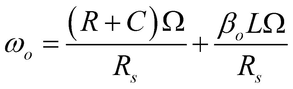
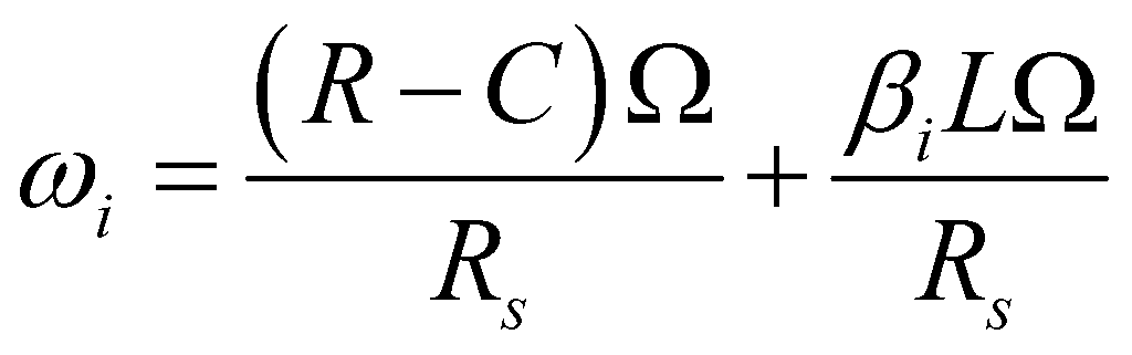
Where R is the radius of turn, to the centre line of the vehicle and Ω is the yaw rate. In these equations the first term on the right hand side is the effect of turning without slip while the second term is the contribution of track slip. The sprocket speed ratio can be shown to be, from Equations (18) and (19):
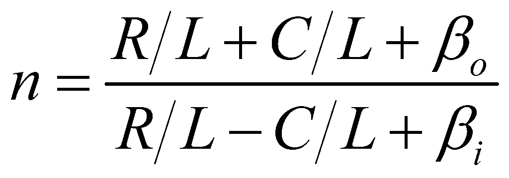
This equation can be rearranged to give:
Radius of turn on hard level ground
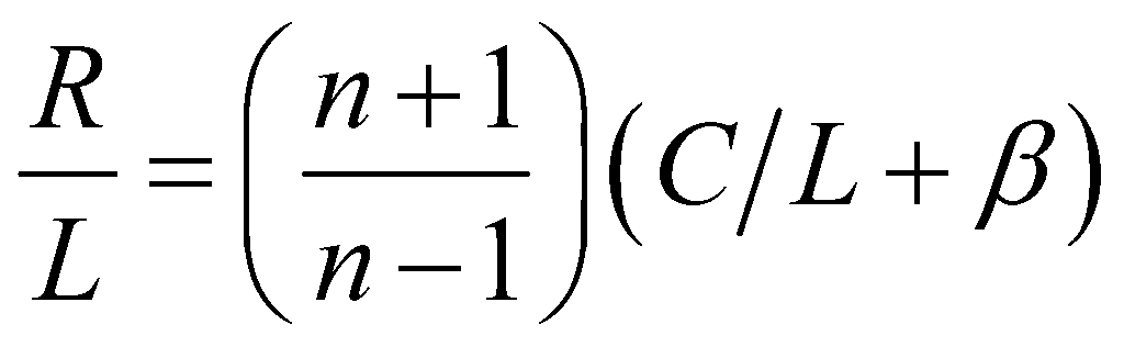
This condition is of particular importance because the vehicle manufacturers commonly quote it and it can be obtained from Equation (21) under the assumption of zero longitudinal load being applied to the vehicle. With this assumption the longitudinal forces generated by the tracks are equal and opposite, with the outer being positive and the inner negative. Thus the same applies for the non-dimensional slip radii. Under this condition Equation (21) becomes:
Engine slip factor
When the vehicle enters a turn, the engine speed may have to change. In considering this aspect the type of steering mechanism needs to be considered. The vast majority of tracked vehicles in current use change the sprocket speeds by equal and opposite amounts, so that the mean sprocket speed maintains the same proportion of engine speed as in the straight ahead condition. Defining the Slip Factor (SF) as the ratio of engine speed with slip to that without, it can be shown that:
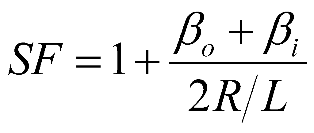
Thus the change in engine speed depends on the slip of the tracks. On hard level ground these will be equal and opposite and the engine speed will remain constant, while in heavy going βo>–βi and the engine speed has to rise to maintain the speed of the vehicle in the turn.
Power required in a turn
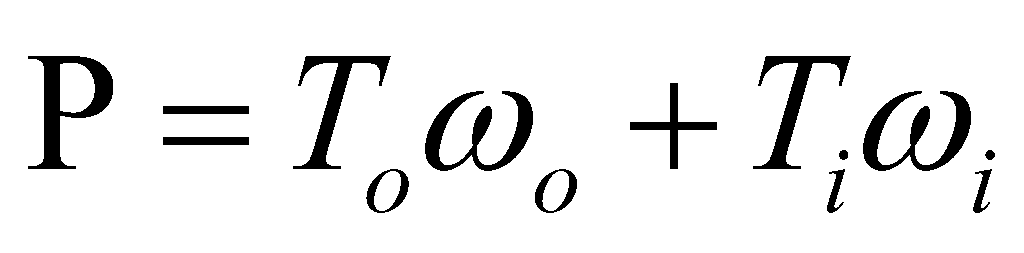
The power required to execute a turn depend on the type of steering mechanism being used, regenerative or non-regenerative. In non-regenerative systems the power input to the inner track is dissipated in the brake on that side and the power required is given by:
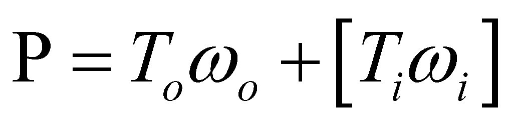
Where the term inside the square brackets is ignored if it is negative.
For a regenerative system the negative power from a slowed inner sprocket is fed to the outer and, assuming 100% transmission efficiency, the total power is given by:
Comparison with experiment
In this section the theoretical model developed is compared to experimental results.
Prediction of sprocket torques
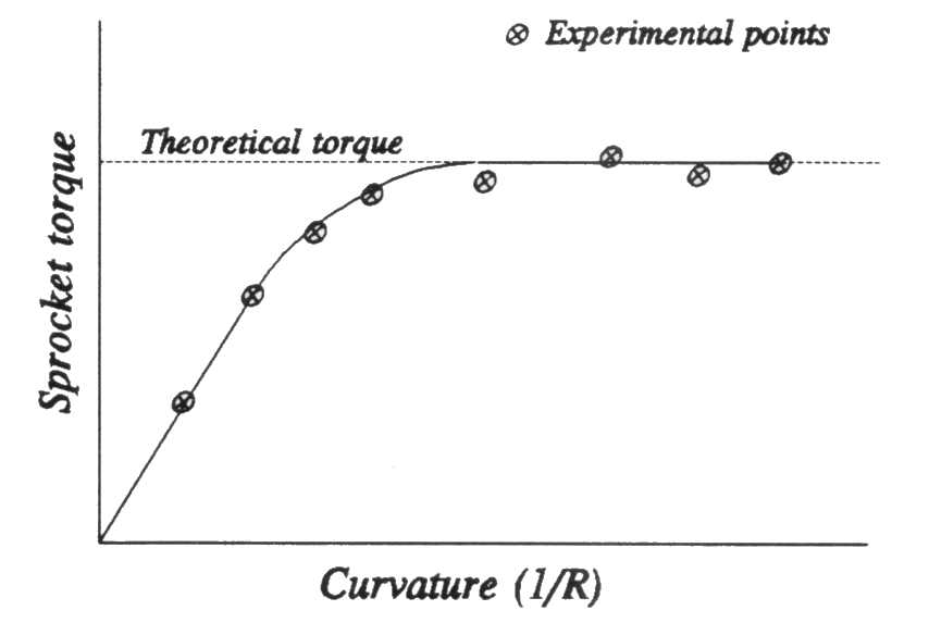
A plot showing the predicted and experimentally measured sprocket torques is shown in Figure 8. In this figure it is seen that for small radii of turn (large curvature) the theory predicts the sprocket torque well, while at large radii it is relatively poor. The main reason for this departure is the rigid track assumption. For a tight turn this is acceptable but not so for a gentle one. The theory thus predicts the maximum inner or outer sprocket torque for a given vehicle geometry, which is important in the design of the transmission.
Prediction of radius of turn
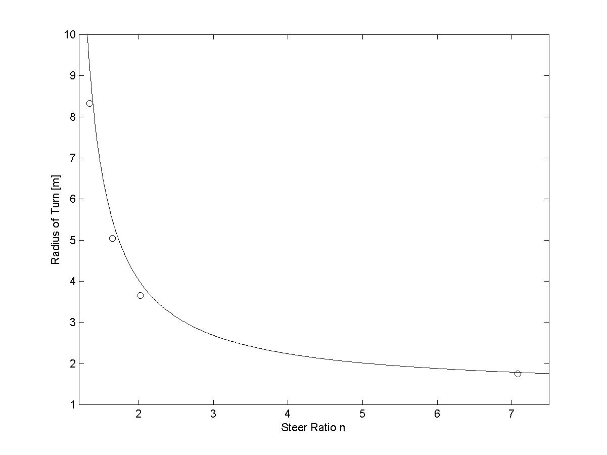
A plot showing the radii of turn against steer ratio for the Combat Vehicle Reconnaissance (Tracked) CVR(T) is shown in Figure 9. The semi-length L and semi-track C are 1.31m and 0.858m respectively. This figure shows the experimentally measured radii of turn for the first four gears, the predicted curve between a steer ratio of 1.3 and 7.5 to compare with. There is good correlation between the measure and predicted radii of turn as shown by the closeness of the predicted to the measured. This figure also shows the initial rapid reduction in radii of turn with steer ratio, which then starts to level out at higher steer ratios.
Using the method
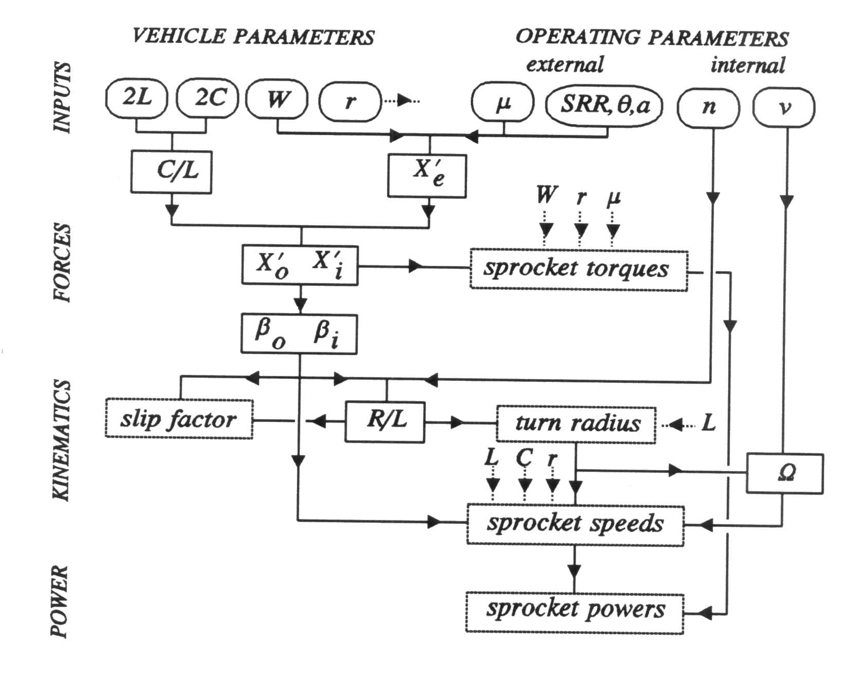
A flow chart for using the method is given in Figure 10. It is important to note that it is necessary to work down the flow chart, even though this may require iteration for some types of problem, for example where it is the available power that is prescribed.
Conclusion
A method of determining the low-speed handling characteristics of skid steer tracked vehicles has been presented. The theory developed is suitable for use by either hand calculation or spreadsheet.
It has been shown that the results predicted by the model for the radius of turn are close to those measured experimentally but only an upper bound is given for the sprocket torque.
References
[1] D. Purdy and P. Wormell, “Handling of High-speed Tracked Vehicles”, Journal of Battlefield Technology, Vol. 6, No. 2, July 2003.
[2] M. Kitano and M. Kuma, “An Analysis of Horizontal Plane Motion of Tracked Vehicles”, Journal of Terramechanics, Vol. 44, No. 4, 1977, pp. 211-225.
[3] J. Wong and C. Chiang, “A General Theory for Skid Steering of Tracked Vehicles on Firm Ground”, Proceedings of the Institution of Mechanical Engineers, Vol. 215, Part D, pp. 343-355.
[4] H. Merritt, “Some Considerations Influencing the Design of High-speed Track-vehicles”, The Institution of Automobile Engineers, January 1939, pp. 398-429.
[5] W. Steeds, “Tracked Vehicles—An Analysis of the Factors Involved in Steering”, Automobile Engineer, April 1950, pp. 143-148.
[6] P. Wormell, Introduction to Skid Steering of Tracked Vehicles, MSc Handout, Royal Military College of Science.
[7] Matlab and Simulink, The MathWorks, Inc, Natick, MA, USA.